
7
Chapter 5 introduced concepts on the origins of surface charge and surface potential, the distribution of dissolved counterions and co-ions in the fluid around a charged surface and their “charge screening” effect, and quantitative expressions for the potential profile (i.e., the decline in potential from the surface potential toward zero potential when moving across the diffuse ion layer and into the bulk fluid). Briefly, higher ionic strength of the fluid yields a higher Debye parameter [latex]\kappa[/latex] and a more rapid decline in the potential energy from the surface. These concepts were all presented for one single surface in a medium. This chapter now extends these concepts to the forces or energies of interaction that develop between two surfaces as they approach. These interaction energies will then be used to predict attachment rates and colloidal stability in Chapter 7.
6.1 Introduction to Interaction Energy Profiles
Interactive Question 6.1: Putt-putt ⛳………….🏌
Imagine yourself on a miniature golf (putt-putt) course with the configurations shown in the activity below. Assume your aim of the golf ball in the direction of the hole is accurate, but you are not sure how hard you need to putt the ball.
Please read these instructions before starting the activity:
- On the first question in the activity, rank the four configurations from the least to highest amount of energy that you would need to provide, in order to putt the ball into the hole.
- On the second question in the activity, consider each position numbered on each diagram (4 positions x 4 diagrams = 16 total positions). If you were to putt the ball to that location, will the ball be stable (i.e., remain at that position) or unstable (i.e., roll away from that position)?
The original version of this chapter contained H5P content. You may want to remove or replace this element.
Why did we do this? This simple concept can translate well to interpreting interaction energy profiles in the remainder of the chapter to follow. The golf ball will represent one particle or surface, and the hole will represent another particle or surface that it is approaching. At the end of this chapter, another quiz will cover real-world examples of the interaction energies discussed here for particle-based systems or products.
Figure 6.1 shows four possible interaction energy profiles for two surfaces approaching each other. You should notice that they are analogous to the four miniature golf configurations in the activity above. The x axis represents the separation distance [latex]h[/latex] between the two surfaces, with a separation distance of [latex]h=0[/latex] indicating direct contact of the two surfaces. The y axis represents the interaction energy [latex]V[/latex] (SI units of J) when the surfaces are brought within separation distance x, normalized to the thermal energy of the system [latex]k_{B}{T}[/latex] (also SI units of J), resulting in the dimensionless ratio, [latex]{V}/{\left(k_{V}{T}\right)}[/latex].
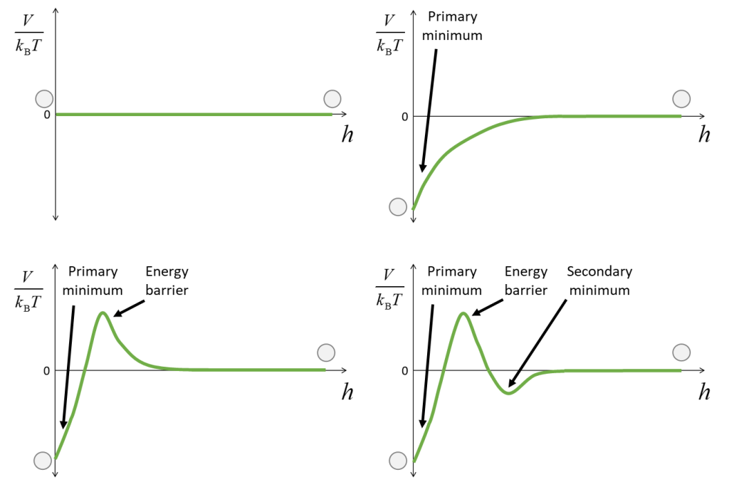
The interpretation of the interaction energy profiles is also analogous to the miniature golf situation. First, it is noted that a positive interaction energy represents an unfavorable state, a negative interaction energy represents a favorable state, and zero interaction energy indicates no interaction. The four scenarios in Figure 3.1 are outlined below:
- No interaction — The top left scenario is not typically encountered but is presented as a theoretical case in which there is no favorable or unfavorable interaction between the two particles or surfaces at any distance, i.e., they cannot “sense” each other.
- In the other three scenarios, there is no interaction at long separation distances, whereas the most favorable and stable energy state (i.e., most negative interaction energy) occurs when particles or surfaces are in direct contact at a separation distance of 0 — this energy well is termed the “primary minimum.” However, the energy profile at intermediate distances (on the order of the Debye length [latex]\kappa^{-1}[/latex]) varies in the three cases:
- Purely attractive interaction — In the top right diagram, there is an increasingly favorable (attractive) interaction as the two particles or surfaces approach, so the two particles will attach in the primary minimum as long as they come within “sensing” distance of each other.
- Repulsive energy barrier — In the bottom left diagram, an energy barrier must be overcome before the particles or surfaces can be brought in direct contact. If a particle has sufficient energy (e.g., thermal energy), it can overcome the barrier and attach in the primary minimum. Otherwise, it will be repelled away from the other surface. The lower the energy barrier, the higher likelihood the particles will have sufficient energy to attach.
- Repulsive energy barrier with a secondary minium — In the bottom right diagram, the energy barrier is preceded by a shallow energy well, termed the “secondary minimum.” Particles with sufficient energy to overcome the energy barrier will attach strongly in the primary mimimum as before. However, those with lower energy can stably reside in the secondary minimum at some small separation distance from each other. Particles that attach in the secondary miminum are only loosely bound, i.e., given some small energy input, they can be separated — for example, the particles may agglomerate when left stagnant but redisperse when shaken.
The remainder of this chapter covers a few common types of attractive or repulsive interactions, and mathematical equations to compute the interaction energy profiles.
6.2 Types of surface interactions
6.2.1 Electrostatic interactions
The electrostatic interaction energy [latex]V_\text{el}[/latex] between two charged surfaces can be attractive (negative energy) for oppositely-charged surfaces, repulsive (positive energy) for like-charged surfaces, or zero for uncharged surfaces. As in Chapter 5, the reader is recommended to explore the colloid science textbooks by Hiemenz and Rajagopalan (1997) and Hunter (2001) for discussion related to the derivation of the interaction energy profiles, along with alternative equations derived under different assumptions. Here, we present equations that have been derived for [latex]V_\text{el}[/latex] with different surface geometries (Figure 6.2). In all three cases, the fluid contains a symmetric electrolyte with bulk ion number concentration [latex]n_{\infty}[/latex] and valence [latex]z[/latex], Debye parameter [latex]\kappa[/latex]), and electric permittivity [latex]\varepsilon=\varepsilon_{\text{r}}\varepsilon_{0}[/latex].
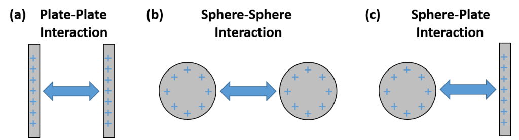
First, two identical surfaces or particles are considered. Equation 6.1 applies for the plate-plate geometry (two flat surfaces, each with surface potential [latex]\psi_0[/latex]), and Equation 6.2 for the sphere-sphere geometry (two spherical particles, each with surface potential [latex]\psi_0[/latex] and radius [latex]R_\text{s}[/latex]). The sphere-sphere interaction is typically applied when considering homo-agglomeration within a sample of particles. It is noted that two equivalent forms are provided for Equation 6.2 depending on whether one groups parameters as [latex]\kappa[/latex] or leaves them separate.
| [latex]{{V}_{\text{el}}}=64{{k}_{\text{B}}}T{{n}_{\infty}}{{\kappa}^{-1}}{{\left[\tanh\left(\frac{ze{{\psi}_{0}}}{4{{k}_{\text{B}}}T}\right)\right]}^{2}}\exp\left(-\kappa h\right)[/latex] | Electrostatic interaction energy, plate-plate geometry, identical surfaces (6.1) |
| [latex]{{V}_{\text{el}}}=64\pi{{R}_{\text{s}}}{{k}_{\text{B}}}T{{n}_{\infty}}{{\kappa}^{-2}}{{\left[\tanh\left(\frac{ze{{\psi}_{0}}}{4{{k}_{\text{B}}}T}\right)\right]}^{2}}\exp\left(-\kappa h\right)[/latex] or [latex]{{V}_{\text{el}}}=64\pi{{\varepsilon}_{0}}{{\varepsilon}_{\text{r}}}\left(\frac{{{R}_{\text{s}}}}{2}\right){{\left(\frac{{{k}_{\text{B}}}T}{ze}\right)}^{2}}{{\left[\tanh\left(\frac{ze{{\psi}_{0}}}{4{{k}_{\text{B}}}T}\right)\right]}^{2}}\exp\left(-\kappa h\right)[/latex] |
Electrostatic interaction energy, sphere-sphere geometry, identical particles (6.2) |
Equations can also be derived for the interactions of two non-identical different surfaces. Equation 6.3 is given below for a sphere-plate interaction, with [latex]\psi_{0,1}[/latex] representing the surface potential of one surface and [latex]\psi_{0,2}[/latex] the other surface. This scenario can be applied to the attachment of nanoparticles or colloids onto much larger particles where the radius of curvature is relatively large and can be approximated as a flat surface (e.g., deposition onto sand grains or glass beads in a packed bed experiment).
| [latex]{{V}_{\text{el}}}=64\pi\left(2{{R}_{\text{s}}}\right){{k}_{\text{B}}}T{{n}_{\infty}}{{\kappa}^{-2}}{{\psi}_{0,1}}{{\psi}_{0,2}}\exp\left(-\kappa h\right)[/latex] or [latex]{{V}_{\text{el}}}=64\pi{{\varepsilon}_{0}}{{\varepsilon}_{\text{r}}}{{R}_{\text{s}}}{{\left(\frac{{{k}_{\text{B}}}T}{ze}\right)}^{2}}{{\psi}_{0,1}}{{\psi}_{0,2}}\exp\left(-\kappa h\right)[/latex] |
Electrostatic interaction energy, sphere-plate geometry, non-identical surfaces (6.3) |
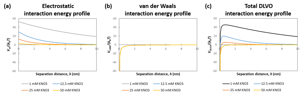
Similarly to the exponential decline of the electric potential with distance from the surface, discussed in Chapter 5, there is also an exponential decline in the electrostatic interaction energy with separation distance [latex]h[/latex] in Equations 6.1 to 6.3. The impact of the dissolved ion concentration and ion valence are captured in the [latex]n_{\infty}[/latex], [latex]z[/latex], and [latex]\kappa[/latex] (which increases with ionic strength). The appearance of [latex]\kappa[/latex] in the [latex]\exp\left(-\kappa h\right)[/latex] term in all three equations is further emphasized. This expression captures the “charge screening” effect, where higher dissolved salt in the solution counters the surface potential and results in weaker electrostatic interaction energies between two charged surfaces. Figure 6.3(a) at the end of this chapter shows computed electrostatic interaction energy profiles for citrate-stabilized gold nanoparticles interacting with themselves at varying ionic strength.
6.2.2 Van der Waals interactions
If two surfaces experienced only electrostatic interactions, then neutral surfaces would have no interaction and like-charged surfaces (e.g., a sample containing particles of the same material) would have purely repulsive interactions; hence, no agglomeration would be expected to ever occur in these situations. However, this is not typically the case. Therefore, there must be a second force between the particles — this is the van der Waals (vdW) interaction.
vdW interactions apply to all molecules and materials and can be sub-classified into Keesom, Debye, and London interactions. The vdW forces arise from the polarity or polarizability of the bonds comprising the molecule or material, and the three classes depend on whether the interactions are between permanent dipoles or induced or instantaneous dipoles, as described below in order from strongest to weakest interaction:
- Keesom interactions — Keesom interactions occur between two species with permanent dipoles. To predict whether a permanent dipole will exist, one can review an electronegativity chart of the atoms in the periodic table. The higher the Pauling electronegativity value, the more strongly the atom draws electrons. When comparing two atoms as in a covalent bond, a higher difference in electronegativity results in a higher dipole moment wherein electrons reside more closely toward the more electronegative atom. If the electronegativity difference is > 1.7, an electron will fully transfer from one atom to the more electronegative atom; fully ionic species will participate in the electrostatic interactions covered in Section 6.2.1 above. On the other hand, an elecronegativity difference between 0.4 and 1.7 yields a polar covalent bond, i.e., a permanent dipole, where the more electronegative atom takes on a partially negative character. When two interacting molelcules or particles both have permanent dipoles, the dipoles can align to yield a favorable (attractive) interaction between the negative and positive ends of the two dipoles. The strength of the Keesom interaction depends on the polarity of the dipoles; hydrogen bonding represents an especially strong Keesom interaction wherein H (low electronegativity) is bonded to O, N, or F (high electronegativity), e.g., as in H2O.
- Debye interactions — Debye interactions occur between a permanent dipole that induces a dipole in a nonpolar species (electronegativity difference < 0.4). For all atoms, the electrons are constantly in motion around the nucleus, and their spatial distribution can change in response to an external force. When a permanent dipole approaches another compound, it can induce a temporary change in the electron distribution (induced dipole), uponwhich the permanent and induced dipole experience an attractive interaction between the negative and positive regions. These interactions are hence also attractive but weaker than the Keesom interactions. The strength of the Debye interaction depends on both the polarity of the permanent dipole and the polarizability of the nonpolar species, i.e., the ease of shifting the electron distribution in response to an external force.
- London interactions — London interactions occur between two nonpolar species where a random shift in electron distribution results in instantaneous dipole, that can temporarily induce another dipole. This instantaneous-induced dipole interaction is a weak attractive interaction. The strength of the London interaction depends on the polarizability of the two species.
The sum of all three classes of interactions yields the vdW interaction energy, first presented for two identical molecules (not surfaces), denoted molecules “1” and “1,” interacting across a vacuum (Equation 6.4):
| [latex]{{V}_{\text{VdW}}}=-\frac{1}{{{\left( 4\pi {{\varepsilon }_{0}} \right)}^{2}}}\left( \frac{2\mu _{1}^{4}}{3{{k}_{\text{B}}}T}+2{{\alpha }_{0,1}}\mu _{1}^{2}+\frac{3}{4}{{h}_{\text{Planck}}}{{\upsilon }_{1}}\alpha _{0,1}^{2} \right){{h}^{-6}}=-{{\beta }_{11}}{{h}^{-6}}[/latex] | vdW interaction energy for two identical molecules interacting over vacuum (6.4) |
where [latex]\mu _{1}[/latex] is the dipole moment of molecule “1” and [latex]\alpha _{0,1}[/latex] is the polarizability of molecule “1.” The first, second, and third terms being summed hence represent the Keesom, Debye, and London interactions, respectively. The multiplicative term on the separation distance can be grouped into one term, [latex]{{\beta }_{11}}[/latex].
When two identical flat surfaces of material “1” and “1” are aligned with the surfaces parallel to each other and all vdW interactions are integrated over an interaction area [latex]A_{\text{int}}[/latex], the vdW interaction energy across vacuum is given by Equation 6.5.
| [latex]{{V}_{\text{VdW}}}=-{{\left( \frac{\rho {{N}_{\text{A}}}}{M} \right)}^{2}}\left( \frac{{{\beta }_{11}}\pi }{12} \right){{A}_{\text{int}}}{{h}^{-2}}[/latex] | vdW interaction energy for two identical surfaces interacting over vacuum (6.5) |
where [latex]\rho[/latex] is the material density (units of mass volume-1), [latex]M[/latex] is the molar mass (mass moles-1), and [latex]N_{\text{A}}[/latex] is Avogadro’s number (moles-1). Grouping terms here yields the Hamaker constant [latex]A_{11}[/latex] for two identical materials interacting across a vacuum.
Typically, materials are not interacting across a vacuum. The Hamaker constant then needs to be adjusted to account for the effect of the intervening medium. Equations 6.6 and 6.7 can be used to compute the Hamaker constant [latex]A_{212}[/latex] for two surfaces of the same material “2” and “2” interacting across medium “1,” or [latex]A_{213}[/latex]two surfaces of different materials “2” and “3” interacting across medium “1.” In either case, one would first look up the Hamaker constant for each material interacting with itself over vacuum (i.e., [latex]A_{11}[/latex], [latex]A_{22}[/latex], and [latex]A_{33}[/latex]) to use in the equations.
| [latex]{{A}_{212}}={{\left( \sqrt{{{A}_{11}}}-\sqrt{{{A}_{22}}} \right)}^{2}}[/latex] | Hamaker constant for two identical surfaces “2” interacting over medium “1” (6.6) |
| [latex]{{A}_{312}}=\left( \sqrt{{{A}_{33}}}-\sqrt{{{A}_{11}}} \right)\left( \sqrt{{{A}_{22}}}-\sqrt{{{A}_{11}}} \right)[/latex] | Hamaker constant for two non-identical surfaces “2” and “3” interacting over medium “1” (6.7) |
Finally, equations for the overall van der Waals interaction energy are provided for surfaces of different geometries — plate-plate, sphere-sphere, and sphere-plate (Figure 6.2) — in Equations 6.8, 6.9, and 6.10, respectively. In these equations, [latex]A[/latex] represents whichever Hamaker constant accurately matches the situation (e.g., [latex]A_{212}[/latex] or [latex]A_{213}[/latex] for the same or different surface materials, respectively, interacting across medium “1”):
| [latex]{{V}_{\text{VdW}}}=-\frac{A}{12\pi }{{A}_{\text{int}}}{{h}^{-2}}[/latex] | vdW interaction energy for plate-plate interactions (6.8) |
| [latex]{{V}_{\text{VdW}}}=-\frac{A}{12}\left( \frac{{{R}_{\text{s,}1}}{{R}_{\text{s,}2}}}{{{R}_{\text{s,}1}}+{{R}_{\text{s,}2}}} \right){{h}^{-1}}[/latex] | vdW interaction energy for sphere-sphere interactions (6.9) |
| [latex]{{V}_{\text{VdW}}}=-\frac{A}{6}{{R}_{\text{s}}}{{h}^{-1}}[/latex] | vdW interaction energy for sphere-plate interactions (6.10) |
Although the van der Waals interaction energy can be repulsive (positive value) in some unusual cases depending on the relative Hamaker constants for the media and the two surface materials), for the vast majority of scenarios, it will be an attractive interaction (negative interaction energy), with the interaction strength declining by a power-law function with increasing separation distance between the two interacting surfaces. The estimated van der Waals interaction energy profile computed for gold nanoparticles interacting across water is shown in Figure 6.3(b) at the end of this chapter.
6.3 Derjaguin-Landau-Verwey-Overbeek (DLVO) Theory
6.3.1 DLVO theory for combined van der Waals and electrostatic interactions
DLVO theory is a framework to estimate the combined effect of multiple forces by taking each relevant interaction energy profile to be additive. In all cases, the van der Waals interaction energy [latex]V_{\text{vdW}}[/latex] must be considered; for charged particles, [latex]V_{\text{el}}[/latex] must also be considered (whereas [latex]V_{\text{el}} = 0[/latex] for uncharged particles). The DLVO equation is hence presented as Equation 6.11:
| [latex]{{V}_{\text{DLVO}}}={{V}_{\text{VdW}}}+{{V}_{\text{el}}}[/latex] | DLVO interaction energy between two surfaces (6.3) |
Exercise 6.1: DLVO computation for gold nanoparticles at different ionic strength
The spreadsheet linked here (DLVO Calculation Template) contains material and system properties for gold nanoparticles. Four salt solutions are considered on the four spreadsheet tabs: 1 mM KNO3, 12.5 mM KNO3, 25 mM KNO3, and 50 mM KNO3.
Complete the spreadsheet as follows:
- In the orange columns on the first spreadsheet tab: Input the appropriate formulae to compute the electrostatic and van der Waals interaction energies at the separation distances listed, and the DLVO interaction energy as the sum of [latex]V_{\text{el}}[/latex] and [latex]V_{\text{vdW}}[/latex].
- In the green columns on the first spreadsheet tab: Normalize the interaction energies by [latex]k_{\text{B}}T[/latex].
- In the second, third, and fourth spreadsheet tabs: Copy your formulae from the first spreadsheet tab.
The figure should autopopulate once you have completed all columns. The plots are presented in Figure 6.3 below to check your calculations.
6.3.2 Extended DLVO theory and impacts of macromolecular adsorbates
The plot generated in the exercise above exhibits the most typical interaction energy profile for two like-charged particles with electrostatic and van der Waals interactions. Notably, as the salt concentration in the media increases, the surface charges are screened, resulting in a diminishing height of the energy barrier. When the energy barrier is low relative to the thermal energy [latex]k_{\text{B}}T[/latex], the particles will have a higher likelihood to be able to cross the energy barrier and attach to each other in the primary minimum ([latex]h = 0[/latex]). As the salt concentration continues to increase, [latex]V_{\text{el}}[/latex] will trend toward zero, such that the overall interaction is completely dominated by the attractive van der Waals interaction. That is, any particle that is only electrostatically stabilized will eventually be destabilized (i.e., they will agglomerate) in high salt solutions. However, electrostatic and van der Waals interactions are not the only types of forces possible.
Extended DLVO theory is a catchall term for extensions of DLVO theory that incorporate other forces beyond electrostatic and van der Waals interactions. Here, we focus on interactions that arise when a particle has an adsorbed layer of macromolecules (e.g., polymers or proteins). This case is relevant in both natural systems, where nanoparticles can gain an adsorbed layer of natural macromolecules such as humic acids or proteins from their environment, and engineered systems, where nanoparticles can intentionally be coated with polymers. The adsorbed molecules can impact the particle interactions in several ways:
- Osmotic forces — In osmosis, a difference in solute concentration drives the motion of solvent molecules from the high concentration reservoir to the low concentration reservoir; this is an entropic process. When polymers attach to form an adsorbed layer on a particle, they form a more concentrated region of polymer “solute” in the fluid around the particles. Bringing two coated particles toward each other will require overlap or compression of the polymer layers, increasing the polymer concentration in the region between the two particles. To alleviate the increased osmostic pressure, the solvent (e.g. water) will tend to move into the overlap region and drive the two particles apart. It is noted that if the background solvent itself contains a higher concentration of dissolved polymer than that in the coating layer, then the opposite phenomenon will occur where it is more favorable for the polymer layers to overlap between the particles, resulting in “depletion flocculation.”
- Enthalpic forces — Intermolecular interactions will change the enthalpy of a system. In the case of polymer coatings, one can consider how much the polymer “likes” to interact with itself or with the solvent. For example, hydrophobic polymers will have much less favorable interactions with water than hydrophilic polymers. The miscibility of polymer with a solvent can be described by the Flory-Huggins [latex]\chi[/latex] parameter that incorporates both the enthalpy of interaction and the entropic tendency for mixing. When [latex]\chi < 1/2[/latex], the solvent is a “good” solvent for the polymer, i.e., the polymer molecules are miscible in the solvent. In contrast, the solvent is a “poor” solvent when [latex]\chi > 1/2[/latex], such that the polymer and solvent will phase separate so that the polymer only interacts with itself. In the “good” solvent case case, overlap of the polymer layers between two approaching particles is unfavorable, whereas in the “poor” solvent case, the polymer overlap is favorable. Hence, the enthalpic force can either discourage or encourage particle agglomeration, depending on the specific type of polymer and solvent.
- Elastic forces — Because the matter from one polymer layer and another cannot occupy the same exact space, the layers must typically become compressed when two coated particles approach and the layers start to overlap. Similar to compressing a spring, an elastic force can arise that opposed the compression of the polymer layers, driving the particles apart. The strength of this force will depend on the stiffness or flexibility of the polymer and its ability to rearrange within the available volume.
- Electrostatic forces — If the polymer is charged, it will impart electrostatic forces in addition to those that may arise from the particle surface itself. If the charge sign of the polymer is the same as that on the particle or if the particle is neutral, the electrostatic forces imparted by the polymer will be repulsive. However, if the polymer is oppositely charge, depending on the concentration and adsorbed amount, the particle charge can be neutralized (destabilizing the particles) or charge reversal can occur (which could result in stabilization if the ultimate magnitude of the charge is high).
If the overall effect of the polymer is to discourage particle attachment, the particles are said to be stabilized by “steric repulsion” or “electrosteric repulsion” in the case of charged coatings where the impact of the electrostatic and steric forces is synergistic (i.e., greater than summative). Of particular note, the steric interaction energies are very strong and are generally not impacted by the salt concentration in the fluid. Therefore, polymer coatings are frequently used in nanoparticle or colloid formulations to achieve products with good dispersibility, even in high ionic strength backgrounds where the particles would lose their electrostatic stabilization. Steric interaction energies are challenging to estimate quantitatively; however, equations have been derived by Vincent et al. (1986) for an uncharged adsorbed layer with a homogeneous polymer density throughout the volume of the layer.
Two other polymer- or adsorbate-induced phenomena are briefly highlighted, wherein the surface coating can enhance rather than diminish the particle agglomeration:
- Bridging flocculation — Occurs when a long polymer chain attaches not just onto one particle, but two or more.
- Patch-charge attraction — Occurs when a charged adsorbate forms a non-uniform coating on an oppositely-charged particles, resulting in both positive and negative patches on the particle surface. When two particles approach, the positive patches on one particle can align with the negative patches on another, resulting in agglomeration.
6.3.3 Real-world examples of particle-particle interaction forces
Interactive Question 6.2: Identify the relevant interaction phenomenom
For each of the scenarios in the following question set, identify which type of interaction (electrostatic interactions, steric repulsion, or bridging flocculation) is predominantly responsible for the observed behavior. Note that van der Waals forces (not listed as a selection option) will always be present in all cases.
The original version of this chapter contained H5P content. You may want to remove or replace this element.