
6
In addition to particle size, which was shown to influence its diffusion and sedimentation rates in Chapter 4, surface charge or surface potential is another property that is important to characterize to understand how a nanoparticle will behave in a liquid suspension. Notably, the colloidal stability of a nanoparticle suspension (i.e., whether the particles remain well-dispersed or agglomerate with each other) and interactions with other surfaces (e.g., whether the nanoparticles stick to the walls of a container) often depend on the sign and magnitude of charge on the particle surface. This chapter covers the origins of surface charge and its relationship to surface potential, as well as the potential profile that develops away from the particle surface. Chapter 5 and Chapter 6 discuss electrostatic forces associated with surface charge and their influence on particle attachment rates, respectively. Finally, Activity 2 demonstrates these phenomena using two types of nanoparticles: citrate-stabilized gold nanoparticles (synthesized in Activity 1) and titanium dioxide nanoparticles.
5.1 Overview of charge (electrostatic) interactions
Exercise 5.1: Balloons 🎈
Watch the YouTube video “Repelling Balloons” by Science Mom (2020).
1. What specific factor determines whether the interactions between two balloons, or a balloon with another suface, will be attractive or repulsive?
2. What factors influence the strength of the interaction between two surfaces?
Why did we watch this? The general concepts in the balloon demo will reappear below and can serve as a good reminder of the phenomena that can be expected when considering interactions between two particles.
5.2 Surface charge and the interfacial structure
Interactions or forces that arise due to surface charge are termed “electrostatic” interactions. As highlighted in the first question in Exercise 5.1 above, when two charged surfaces interact, their charge signs (positive or negative) determines whether the electrostatic interaction is attractive (oppositely-charged surfaces) or repulsive (like-charged surfaces). Here, we consider the chemistry of how a surface can develop charge, whether the charge will be positive or negative or if there will be be no charge, i.e., a neutral surface, and the structure of charged species at the particle surface.
5.2.1 Surface charge derived from interactions of metal oxides in water
First, we will consider metal oxide materials, for example, titanium dioxide (TiO2) or silicon dioxide (SiO2). For crystalline materials, each atom in the interior of the particle is situated within a lattice in which it bonds in a repeating pattern with its neighboring atoms. Throughout the interior or bulk of the material, the metal oxide material is uncharged, with the positive oxidation state of the metal atom (e.g., +4 for Ti in TiO2) balanced by the negative oxidation state of the oxygen atoms (‑2). However, metal atoms at the surface of the particle (denoted “≡Me”, with “≡” representing the bonding to the bulk solid material) are lacking one or more bonds to oxygen where the material is cleaved, resulting in an energetically unfavorable state and a Lewis acid character. That is, the surface metal atom will accept electrons from a Lewis base. When placed into water, these sites can make up this interaction by adsorbing water molecules at the surface; or more commonly, the water molecule will dissociate, releasing H+ into solution while the OH– group from the water molecule chemically bonds (“chemisorbs”) to the metal atom, forming a surface hydroxyl group (≡MeOH).
The (≡MeOH) group exhibits weak acid or weak base properties — either dissociating to lose H+, resulting in a negatively charged surface oxide group (≡MeO‑); or gaining another H+, resulting in a positively charged surface ≡MeOH2+ group, as shown in Figure 5.1.
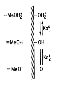
DOI:10.1021/ba-1980-0189.ch001. Copyright 1980, American Chemical Society)
As with the weak acid/base chemistry described in Activity 1 for dissolved molecules, each protonation or deprotonation event for the surface sites has an acid dissociation constant [latex]K_{\text{a}}^{\text{s}}[/latex] for the dissociation reaction of the acid form (HA) to the base form (A–), i.e., HA ⇋ H+ + A– (Figure 5.1). The equilibrium between the products and reactants is given by Equation 5.1 below. Equation 5.1 can also be rearranged to the Henderson-Hasselbalch equation by applying the relationships [latex]\text{p}K_{\text{a}}^{\text{s}}=-{{\log }_{10}}K_{\text{a}}^{\text{s}}[/latex] and [latex]\text{pH}=-{{\log }_{10}}\left\{{\text{H}}^{+}\right\}[/latex], resulting in Equation 5.2.
| [latex]K_{\text{a}}^{\text{s}}=\frac{\left\{ {{\text{H}}^{+}} \right\}\left\{ {{\text{A}}^{-}} \right\}}{\left\{ \text{HA} \right\}}[/latex] | Acid dissociation constant (5.1) |
| [latex]\text{pH}=\text{p}K_{\text{a}}^{\text{s}}+{{\log }_{10}}\frac{\left\{ {{\text{A}}^{-}} \right\}}{\left\{ \text{HA} \right\}}[/latex] | Henderson-Hasselbalch equation (5.2) |
If multiple deprotonation events can occur (e.g. ≡MeOH2+ ⇋ ≡MeOH + H+, followed by ≡MeOH ⇋ ≡MeO‑ + H+), there are two separate [latex]\text{p}K_{\text{a}}^{\text{s}}[/latex] values for each event — e.g., [latex]\text{p}K_{\text{a,1}}^{\text{s}}[/latex] for the first deprotonation, and [latex]\text{p}K_{\text{a,2}}^{\text{s}}[/latex] for the second deprotonation.
As can be determined from either Equation 5.1 or 5.2, when the solution pH is equal to [latex]\text{p}K_{\text{a}}^{\text{s}}[/latex], the conjugate acid (HA) and conjugate base (A‑) forms are present at equal concentrations. Furthermore, while the pH is near [latex]\text{p}K_{\text{a}}^{\text{s}}[/latex] (i.e., within 1 or 2 pH units above or below the [latex]\text{p}K_{\text{a}}^{\text{s}}[/latex] value), the sample will have a mixture of the acid and base forms (e.g. if the pH is 1 pH unit below [latex]\text{p}K_{\text{a}}^{\text{s}}[/latex], then 90% will be in the acid form and 10% in the base form. If the pH is far from the [latex]\text{p}K_{\text{a}}^{\text{s}}[/latex], then one form will dominate and the other can be considered negligible.
5.2.2 Point of zero charge
A simpler way to understand the charge state of a surface is the “point of zero charge” (pzc). As discussed above, the sites on a metal oxide surface can undergo two transitions as the pH increases, from positively-charged ≡MeOH2+ to neutral ≡MeOH to negatively-charged ≡MeO‑. When the pH reaches pKa,1, there are equal amounts of the ≡MeOH2+ and neutral ≡MeOH forms, i.e., the surface has a moderate positive charge. When the pH reaches pKa,2, there are equal amounts of the ≡MeOH and ≡MeO‑ forms, i.e., the surface has a moderate negative charge.
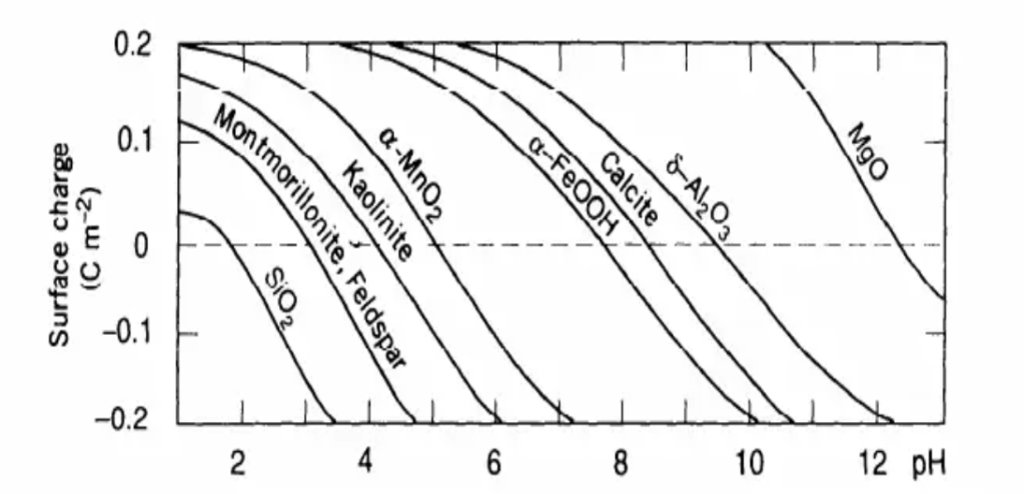
Rather than specifying the two pKa values, it can be more straightforward to simply identify at what pH the surface has a net neutral charge, i.e., the sites are either predominantly in the MeOH form or there are equal quantities or the ≡MeOH2+ and ≡MeO‑ forms. The pH value corresponding to the net neutral surface charge is the pzc and occurs exactly in between pKa,1 and pKa,2. The net surface charge density [latex]\sigma[/latex] (units of charge length-2, e.g., C m-2, where 1 electron carries an elementary charge, e, of 1.602 × 10⁻¹⁹ C) at different pH values and the point of zero charge can be experimentally determined by titration, analogous to titration experiments on dissolved acid/based compounds. Note that a positive or negative value of [latex]\sigma[/latex] denotes a positively- or negatively-charged surface, respectively.
The utility of the pzc should be clear when viewing plots of the surface charge as a function of pH, as shown in Figure 5.2 below. The pzc is the pH value (along the x axis) where [latex]\sigma = 0[/latex], i.e., the transition point from net positive to net negative surface charge.
Interactive Question 5.1: Surface charge of metal oxide materials
The original version of this chapter contained H5P content. You may want to remove or replace this element.
5.2.3 Surface charge derived from adsorbing species
In Activity 1, gold nanoparticles were synthesized using an aqueous medium containing sodium citrate. In this case, the gold atoms are in the zerovalent state (Au0) and form a pure gold nanoparticle rather than a metal oxide. Therefore, a gold nanoparticle should hypothetically develop no surface charge in water. However, as discussed in Activity 1, a citric acid molecule (H3Cit0) undergoes three deprotonations at progressively higher pH to H2Cit‑1, HCit‑2, and Cit‑3. The adsorption of negatively charged citrate species on the gold surface hence imparts the surface charge.
In general, any type of charged species that adsorbs to any type of particle (charged or uncharged) could impart its charge to the particle surface. Charged adsorbates could include a variety of species, with some examples given in Table 5.1 (for the organic species having a charged functional group, “R” denotes the rest of the molecule to which the group is bonded).
| Class of species | Examples |
| Inorganic cations | Na+, Ca2+, Fe3+; will contribute positive charge upon adsorbing |
| Inorganic anions | Cl‑, SO42‑, PO43‑; will contribute negative charge upon adsorbing |
| Organic cations | Weak base compounds, e.g. amines (R–NH2 for primary amines); will contribute positive charge when pH < pKa of the conjugate acid (typically, pKa is between 10 to 11 for primary amines, and can be looked up for other types of weak bases) |
| Organic anions | Weak acid compounds, e.g. carboxylic acids (R–COOH); will contribute negative charge when pH > pKa of the acid (typically, pKa is between 4 to 5 for carboxylic acids and can be looked up for other types of weak acids)
Strong acid compounds, e.g. sulfonates (R–SOO–); will contribute negative charge at any typical pH (pKa < 0 for strong acids) |
Some additional classes of charged species of note besides the simple cases provided in the table are polyelectrolytes and zwitterions. Polyelectrolytes are polymers in which the monomer species comprising the polymer have an acid or base group, for example, polysytrene sulfonate. A large polyelectrolyte molecule can carry a very large number of charges for each monomer that deprotonates or protonates. Zwitterions are charged species with equal numbers of positive and negative charges; for example, an amino acid at a pH in between the pKa of the carboxylic acid group and the pKa of the amine group. Although the zwitterion has a net neutral charge, separate interactions can occur with the two separately charged groups.
Besides the type of species, adsorbates can also be classified by how closely they are associated with the particle surface. These distinctions are discussed in the following section.
5.2.4 The interfacial region
The particle surface, adsorbates on the surface, and ions that accumulate in the fluid near the surface form a structure termed the “electrical double layer.” Two ways of presenting the surface are shown in Figure 5.3 and Figure 5.4. Figure 5.3focuses on classifying the surface functional groups and adsorbate species, based on how they associate with the surface; the definitions below follow those presented by Stumm (1995).
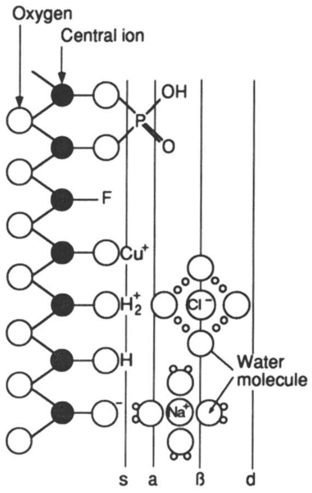
- The bottom three species in the diagram are the surface hydroxyl groups (defining the plane denoted “s” in the diagram) in the three charge states, as discussed in Section 5.2.1.
- Moving up the surface, a Cu2+ ion has displaced H+ from the surface ≡MeOH and is adsorbed directly at the surface at the oxygen atom; these types of complexes are termed “inner-sphere complexes.” At the top of the figure, an F– ion and PO43- ion have adsorbed directly to the ≡Me, also displacing the oxygen; these complexes are a more specific subset of inner-sphere complexes, denoted “ligands.” The layer containing the inner-sphere complexes is labeled “a” in Figure 5.3. When a complexation interaction occurs, the adsorption can also be classified as “specific adsorption,” denoting that there is an attraction beyond simply a charge interaction.
- Moving away from the surface into the liquid, a positive Na+ and negative Cl– ion are shown associating with the negative ≡MeO‑ and positive ≡MeOH2+ surface groups, respectively, corresponding to the attractive electrostatic interaction bewteen oppositely-charged species. Of note however are the molecules of water that surround the ions, forming a hydration shell. Hydrated or solvated ions located immediately at the surface are termed “outer-sphere complexes” and define the layer labeled “β” in Figure 5.3. When ions accumulate at the surface solely by electrostatic interactions, this adsorption can be classified as “non-specific” or “indifferent” adsorption.
- Finally, in the region beyond the outer-sphere complexes but still near the surface, ions can continue to accumulate in a non-random distribution, i.e., with higher concentrations of “counter-ions” having opposite charge to the net surface charge, compared to “co-ions” having the same charge sign. Note that these ions are not drawn in Figure 5.3 but will be the focus of Section 5.3 on the potential profile. These ions are termed “diffuse ions” and reside within the layer labeled “d” in Figure 5.3.
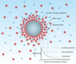
Figure 5.4 focuses on terminology used to name each layer around the particle. Definitions listed below follow Hackley and Ferraris (2001) and are described below in order from closest to furthest distance from the surface.
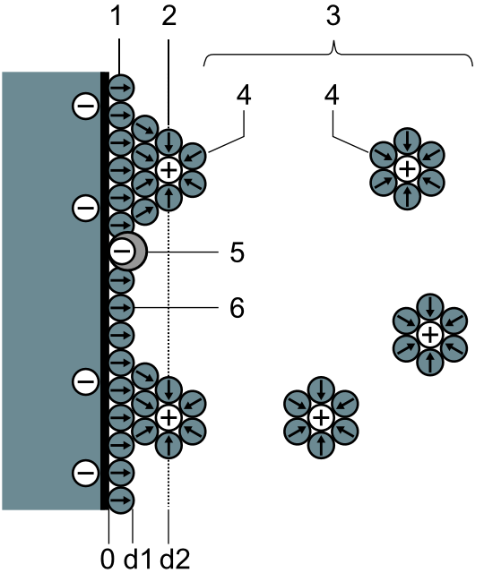
- The Stern layer, also called the inner Helmholtz plane (IHP), includes the inner-sphere complexes that adsorb directly on the particle with no hydration layer between the ion and surface. The Stern layer is depicted as layer “1” at distance “d1” in Figure 5.4 and includes the specifically adsorbed ions “5.”
- The shear plane contains the liquid molecules and any dissolved solutes that remains adhered to the surface as the particle moves through the fluid. The shear plane is often equivalent to the outer Helmholtz plane (OHP), which contains the outer-sphere complexes located at the closest possible distance to the surface while maintaining their hydration layer. The OHP is depicted as layer “2” at distance “d2” in Figure 5.4 and includes the solvated ions “4.”
- The diffuse layer contains the diffuse ions that exhibit non-random distributions (higher counterion versus co-ion concentrations) due to electrostatic interactions with the charged surface; e.g., for a negatively-charged particle in an aqueous medium containing dissolved NaCl, [Na+] > [Cl–] within the diffuse layer. The diffuse layer is depicted as layer “3” in Figure 5.4.
- Finally, the liquid beyond the diffuse layer can be termed the bulk fluid and will have balanced positive and negative charges, e.g., for a particle in an aqueous fluid containing dissolved NaCl, [Na+] = [Cl–] in the bulk fluid.
5.3 Ion distributions, surface potential, and the potential profile
5.3.1 Ion distribution in the diffuse layer
Considering the electrical double layer structure around the particle, it is not only the surface itself that is important in electrostatic interactions, but also what is happening with ions in the fluid layer around the particle. This concept is also related to the second question in Exercise 5.1 above, where the strength of the force between two charged surfaces depended on the distance between the surfaces and the media separating them.
In a physical diagram, the electrical double layer is generally depicted by drawing the counterion and co-ion distributions around the surface — i.e., the number ion concentration [latex]n_{i}[/latex] (units of length-3) for each ion species, i, as a function of distance from the particle surface (Figure 5.5).
Each ion has a valence of [latex]z_{i}[/latex], e.g., [latex]z_{i} = +1[/latex] for monovalent cations, such as Na+; [latex]z_{i} = -1[/latex] for monovalent anions, such as Cl–; [latex]z_{i} = +2[/latex] for divalent cations, such as Ca2+; [latex]z_{i} = -2[/latex] for divalent anions, such as SO42-, and so on. If the cations and anions have equal magnitude of valence — e.g., a solution of NaCl — the electrolyte is considered a “symmetric electrolyte.” If they have different valences — e.g., a solution of CaCl2, the eletrolyte is considered a “non-symmetric electrolyte.” The number concentration of ions is related to the molar concentration [latex]\left[i\right][/latex] by Avogadro’s number [latex]N_\text{A}[/latex]; e.g., for 5 mM NaCl, [latex]{n}_{\text{Cl}}^{-}={N}_{\text{A}}\left[{\text{Cl}}^{-}\right]=\left(6.022\times{10}^{23}\text{ mol}^{-1}\right)\left(0.100\text{ }\frac{\text{mol}}{\text{L}}\right)=6.022\times{10}^{23}\text{ L}^{-1}[/latex].
The charge carried per ion (SI units of C) is computed as [latex]{z_{i}}{e}{n_{i}}[/latex], where [latex]e[/latex] is the elementary charge as noted in Section 5.2.2. The overall charge density [latex]\rho^{*}[/latex] (Si units of C m-3) is then given by Equation 5.3:
| [latex]{{\rho }^{*}}=\sum\limits_{i}{{{z}_{i}}e{{n}_{i}}}[/latex] | Charge density in solution (5.3) |
However, another related property — the electrical potential — is required for calculation of the electrostatic forces of interaction.
5.3.2 Definition of electric potential and surface potential
The electric potential [latex]\psi[/latex] can be defined as the amount of energy required to move a unit of charge from a reference location (where [latex]\psi = 0[/latex]) to the specified location, [latex]x[/latex] (Figure 5.5). The SI units of potential are J/C or V. In the context of a charged surface, the position [latex]x = 0[/latex] is located at the surface, and the reference location is taken far away from the surface ([latex]x\to \infty[/latex]). Hence, the surface potential is denoted [latex]\psi_{0}[/latex]. As with [latex]\sigma[/latex], [latex]\psi[/latex] will have a positive or negative value for a positively- or negatively-charged surface, respectively. [latex]\left|{\psi}\right|[/latex] denotes the absolute value or the magnitude of the potential (always positive). A higher [latex]\left|\sigma\right|[/latex] will correspond to a higher [latex]\left|{\psi}\right|[/latex].
5.3.3 Charge screening and the Debye parameter
When a surface is charged, the charge that it carries must be balanced by the ions in the diffuse layer, with an excess of counterions over co-ions (Figure 5.5). Summing the net charges contained by the surface and the fluid up to a distance [latex]x[/latex] from the surface, the charge is increasingly balanced by the counterions as one moves further and further from the surface until it is ultimately fully balanced. Hence, the magnitude of the potential declines from [latex]\left|\psi\right|=\left|\psi_{0}\right|[/latex] at the surface, to [latex]\left|\psi\right| \to 0[/latex] as one moves across the diffuse layer and into the bulk fluid. This phenomenon is termed “charge screening” and provides the physical explanation of why the electrostatic interaction force declined with distance in Excercise 5.1.
Now, let us consider the impact of the medium around the particle. First, the medium itself will affect how well the potential transmits away from the surface, as described by its electric permittivity, [latex]\varepsilon[/latex] (SI units of F m-1, where 1 F = 1 C/V = 1 J/V2 = 1 C2/J. The electric permittivity is frequently reported as the relative permittivity (or dielectric constant) [latex]\varepsilon_{\text{r}}[/latex], with [latex]\varepsilon=\varepsilon_{\text{r}}\varepsilon_{0}[/latex], where [latex]\varepsilon_{0}[/latex] is the vacuum permittivity (8.854 F m-1). For water, the relative permittivity values at various temperatures have been published by Malmberg and Maryott (1956).
From (Figure 5.5), it is apparent that the salt or electrolyte concentration in the fluid is also important. If a higher overall concentration of ions is available (including counterions), the surface charge will be balanced closer to the surface; i.e., in higher salt, the charge screening effect is stronger. In addition, if the counterion valence is higher (e.g., Ca2+ instead of Na+, screening a negative surface charge), then the charge screening effect is also stronger.
These effects are encapsulated in the Debye parameter [latex]\kappa[/latex], which has units of length-1 (Equation 5.4):
| [latex]\kappa =\sqrt{\frac{{{e}^{2}}}{\varepsilon {{k}_{\text{B}}}T}\sum\limits_{i}{\left( z_{i}^{2}{{n}_{i,\infty }} \right)}}[/latex] | Debye parameter (5.4) |
where [latex]{k}_{\text{B}}[/latex] is the Boltzmann constant and [latex]T[/latex] is the temperature.
The inverse Debye parameter [latex]\kappa^{-1}[/latex] has units of length and therefore, is also called the Debye length. [latex]\kappa^{-1}[/latex] is often reported in nm and serves as a general measure of the distance across which the surface charge is still “felt.” A longer Debye length (smaller Debye parameter) corresponds to longer-ranged electrostatic forces (lower charge screening), whereas a shorter Debye length (higher Debye parameter) corresponds to shorter-ranged electrostatic forces (higher charge screening).
Note on the relationship betwen the Debye parameter and ionic strength: The term “ionic strength” is frequently used in water chemistry and incorporates information on the ion valence and number concentration in a similar form to that in Equation 5.4. The ionic strength [latex]I[/latex] has molar units and is computed as Equation 5.5:
| [latex]I=\frac{1}{2}\sum\limits_{i}{{{C}_{i}}z_{i}^{2}}[/latex] | Ionic strength (5.5) |
where [latex]{C}_{i}[/latex] is the molar concentration of ion [latex]i[/latex]. For monovalent electrolytes, e.g. NaCl, [latex]I[/latex] will be equal to the molar concentration of the salt, e.g., a 0.1 M solution of NaCl yields an ionic strength of 0.1 M. On the other hand, the ionic strength is higher than the salt concentration when multivalent ions are present, e.g., as in CaCl2 or CaSO4. It is left as an exercise to the reader to derive the expression for the Debye parameter in terms of the ionic strength.
5.3.4 Potential profiles
Deriving the mathematical shape of the potential profile, [latex]\psi \left(x\right)[/latex], relies on the combination of the Poisson equation and the Boltzmann factor — yielding the Poisson-Boltzmann equation. The equations and some solutions are provided here without derivation or in-depth discussion; for a thorough presentation of this topic, the reader is referred to the following recommended colloid science textbooks:
- Hiemenz, P. C. and Rajagopalan, R. Principles of Colloid and Surface Chemistry, 3rd ed., 1997, CRC Press: Boca Raton, FL, USA, DOI: 10.1201/9781315274287.
- Hunter, R. J., Foundations of Colloid Science, 2nd ed., 2001, Oxford University Press: Oxford, UK. Available online from Knovel.
In brief, the Poisson equation relaties the potential to the charge density [latex]\rho^{*}[/latex] at a given point (Equation 5.6), and the Boltzmann factor relates the concentration of each ion to the potential at a given point (Equation 5.7):
| [latex]\frac{{{\partial }^{2}}\psi }{\partial {{x}^{2}}}+\frac{{{\partial }^{2}}\psi }{\partial {{y}^{2}}}+\frac{{{\partial }^{2}}\psi }{\partial {{z}^{2}}}=-\frac{{{\rho }^{*}}}{\varepsilon }[/latex] | Poisson equation (5.6) |
| [latex]\frac{{{n}_{i}}}{{{n}_{i,\infty}}}=\exp\left(-\frac{{{z}_{i}}e\psi}{{{k}_{\text{B}}}T} \right)[/latex] | Boltzmann factor (5.7) |
Equations 5.3, 5.6, and 5.7 together result in the Poisson-Boltzmann equation (Equation 5.8):
| [latex]\frac{{{\partial }^{2}}\psi }{\partial {{x}^{2}}}+\frac{{{\partial }^{2}}\psi }{\partial {{y}^{2}}}+\frac{{{\partial }^{2}}\psi }{\partial {{z}^{2}}}=-\frac{e}{\varepsilon }\sum\limits_{i}{\left[ {{z}_{i}}{{n}_{i,\infty }}\exp \left( -\frac{{{z}_{i}}e\psi }{{{k}_{B}}T} \right) \right]}[/latex] | Poisson-Boltzmann equation (5.8) |
This is a partial differential equation, but analytical solutions have been derived under simplifying assumptions. Notably, following the discussion presented by Hiemenz and Rajagopalan (1997), when the potential is low, i.e., [latex]\frac{{{z}_{i}}e\psi }{{{k}_{B}}T}<1[/latex] (the Debye-Hückel approximation), the exponential term in Equation 5.8 can be expanded as a power series and truncated to only the linear term, resulting in the linearized Poisson-Boltzmann equation (Equation 5.9). The right-hand-side of the equation can further be written in terms of the Debye parameter [latex]\kappa[/latex], as also shown in Equation 5.9.
| [latex]\frac{{{\partial }^{2}}\psi }{\partial {{x}^{2}}}+\frac{{{\partial }^{2}}\psi }{\partial {{y}^{2}}}+\frac{{{\partial }^{2}}\psi }{\partial {{z}^{2}}}=\frac{{{e}^{2}}}{\varepsilon {{k}_{B}}T}\sum\limits_{i}{\left( {{z}_{i}}{{n}_{i,\infty }} \right)}\psi ={{\kappa }^{2}}\psi[/latex] | Linearized Poisson-Boltzmann equation, for low potentials (Debye-Hückel approximation) (5.9) |
For a monovalent ions at temperature of 298 K, the condition for a “low” potential can be calculated as [latex]\left|{\psi}\right|<25.7\text{ mV}[/latex]. We will find in the following chapters that this magnitude of potential also serves as a general boundary for whether a particle is electrostatically stabilized (strong charge repulsion) or not.
5.3.4.1 Potential profile for a planar surface with low potentials
In the scenario of a planar surface situated along the [latex]y[/latex] and [latex]z[/latex] directions with homogeneous charge density along the surface, and taking [latex]\psi=\psi_{0}[/latex] at the surface and [latex]\psi \to 0[/latex] for [latex]x \to \infty[/latex], the following solution applies for the potential profile away from the surface under the Debye-Hückel approximation (Equation 5.10):
| [latex]\psi ={{\psi }_{0}}{{e}^{-\kappa x}}[/latex] | Potential profile for a planar surface with low potentials (Debye-Hückel approximation) (5.10) |
Hence, the potential drops off exponentially as one moves from the particle surface across the diffuse ion layer into the fluid. Notably, as the ionic strength of the solution increases, [latex]\kappa[/latex] increases and the potential is screened closer to the surface, resulting in shorter-range electrostatic interactions. It is further noted that when a distance of [latex]x=\kappa^{-1}[/latex] is inputted to Equation 5.10, then [latex]\psi ={{\psi }_{0}}{e}^{-1}=0.37{{\psi }_{0}}[/latex]. That is, at the Debye length, the magnitude of the potential is 37% of the surface potential. Therefore, the Debye length should not be interpreted as the distance where the charge is no longer felt, but it can be useful as a rule of thumb or for comparing situations (e.g. high versus low ionic strength).
5.3.4.2 Potential profile around a spherical particle with low potential
An analytical solution has also been derived for the potential profile around a spherical particle with radius [latex]{R}_{\text{s}}[/latex] and surface potential [latex]\psi_{0}[/latex] in radial coordinates, taking [latex]r = 0[/latex] at the center of the particle, [latex]r = {R}_{\text{s}}[/latex] at the surface of the particle, and [latex]r > {R}_{\text{s}}[/latex] in the fluid around the particle (Equation 5.11):
| [latex]\psi ={{\psi }_{0}}\left( \frac{{{R}_{\text{s}}}}{r} \right){{e}^{-\kappa (r-{{R}_{\text{s}}})}}[/latex] | Potential profile for a spherical particle with low potentials (Debye-Hückel approximation) (5.11) |
Hence, the potential declines exponentially from the surface with the same dependence on [latex]\kappa[/latex] as in the planar case.
5.4 Relationships between surface charge density, surface potential, and zeta potential
In Section 5.3 above, all equations have been presented in terms of the surface potential [latex]\psi_{0}[/latex], whereas Section 5.2 focused on the surface charge density [latex]\sigma[/latex], which can be experimentally measured by titration. This section explores the mathematical relationships between these parameters and another potential — the zeta potential [latex]\zeta[/latex].
5.4.1 Relating surface charge density and surface potential
5.4.2.1 Surfaces with low potentials (Debye-Hückel approximation)
As in Section 5.3, simplifying assumptions are required to derive analytical solutions to relate [latex]\sigma[/latex] to [latex]\psi_{0}[/latex]. If the linearized Poisson-Boltzmann equation applies (i.e., the Debye-Hückel approximation), then Equations 5.12 and 5.13 result for a planar surface and spherical particle, respectively:
| [latex]\sigma =\varepsilon \kappa {{\psi }_{0}}[/latex] | Surface charge density – surface potential relationship for a planar surface with low potential (5.12) |
| [latex]\sigma =\frac{\varepsilon }{{{R}_{\text{s}}}}(1+\kappa {{R}_{\text{s}}}){{\psi }_{0}}[/latex] | Surface charge density – surface potential relationship for a spherical particle with low potential (5.13) |
5.4.2.1 Planar surfaces in symmetric electrolytes (Gouy-Chapman theory)
In the case of a planar surface in a fluid containing a symmetric electrolyte (i.e., [latex]\left|z_{i}\right|[/latex] for the cations is equivalent to that of the anions), it is mathematically possible without invoking the low potential assumption to derive analytical solutions for both the potential profile, i.e., [latex]\psi[/latex] as a function of distance [latex]x[/latex] from the surface (not provided here), along with the relationship between the surface potential and surface charge density as Equations 5.14 and 5.15 for computation of [latex]\sigma[/latex] given [latex]\psi_{0}[/latex] and vice versa, respectively. This derivation is named Gouy-Chapman theory, and the reader is referred to Hiemenz and Rajagopalan (1997) for a textbook presentation of the theory.
| [latex]\sigma ={{\left(8\varepsilon{{k}_{\text{B}}}T{{n}_{\infty}}\right)}^{1/2}}\sinh\left(\frac{ze{{\psi}_{0}}}{2{{k}_{\text{B}}}T} \right)[/latex] | Gouy-Chapman equation for [latex]\sigma[/latex] given [latex]\psi_{0}[/latex] (5.14) |
| [latex]{{\psi}_{0}}=\frac{2{{k}_{B}}T}{ze}\operatorname{asinh}\left[\frac{\sigma}{{{\left(8\varepsilon{{k}_{\text{B}}}T{{n}_{\infty}}\right)}^{1/2}}}\right][/latex] | Gouy-Chapman equation for [latex]\psi_{0}[/latex] given [latex]\sigma[/latex] (5.15) |
It is noted that for the symmetric electrolyte, [latex]z[/latex] in Equations 5.14 and 5.15 is the magnitude of the valence (equivalent for all ions in solution), and [latex]n_{\infty}[/latex] is the number concentration of either the anions or the cations (not the sum of both ions). The functions [latex]\operatorname{sinh}[/latex] and [latex]\operatorname{asinh}[/latex] are the hyperbolic sine function and inverse hyperbolic sine function, respectivley, which can be readily calculated in a spreadsheet program, many programming languages, and some models of scientific calculators.
5.4.2 Zeta potential and the isoelectric point
The titration method to experimentally determine the surface charge density and point of zero charge have been noted in Section 5.2 above. However, in the discussions of the surface potential, experimental methods for their measurement have not been indicated; this is because it is difficult to actually measure the surface potential in practice.
Here, the zeta potential [latex]\zeta[/latex] is now defined as the potential at the shear plane (the boundary where fluid remains adhered on the particle surface when the particle is in motion), i.e., at a location slightly away from the solid particle surface. Therefore, the magnitude of the zeta potential is somewhat lower than that of the surface potential. The zeta potential is of practical importance because, as will be covered in Laboratory 2, common methods to evaluate the potential or charge of a particle or other solid material require motion — either of the particle through the fluid, or the fluid past a fixed solid surface. Therefore, the measured potential corresponds to the zeta potential, rather than the surface potential.
When zeta potential measurements are taken on the same material across different pH values, a plot can be created analogous to that in Figure 5.2. For example, the linked technical Q&A from Malvern Panalytical, a manufacturer of instruments that can measure zeta potential, shows [latex]\zeta[/latex] measurements versus pH for alumina (Al2O3) particles. However, the pH at which [latex]\zeta = 0[/latex] should be reported as the “isoelectric point” (iep) rather than the point of zero charge.