
5
Particle size directly impacts its motion in a fluid. This chapter provides an overview of diffusive motion, motion under a gravitational field, and motion under a centrifugal field. Particle motion in an applied electrical field and an applied flow field are discussed in the chapters on electrophoretic light scattering and field flow fractionation, respectively.
4.1 Brownian motion and the diffusion coefficient
Imagine a cup of water sitting at rest on a table. Even though the bulk of the water is stagnant, the individual molecules of water in the cup are constantly in random motion due to their thermal energy. When a particle is suspended in this fluid, random collisions with the fluid molecules will cause the particle to also undergo random motion, i.e., Brownian motion. The mean square displacement (MSD) of the particle from its initial position, e.g., [latex]\overline{{{x}^{2}}}[/latex] for a particle moving in 1 dimension, will increase proportionally with time [latex]t[/latex] following Equation 4.1 for 1-dimensional motion (back and forth along a line). Equations 4.2 and 4.3 are also provided for 2-dimensional motion (across a flat plane) and 3-dimensional motion (through a volumetric space) using Euclidean coordinates, x, y, and z.
| [latex]\text{MSD}=\overline{{{x}^{2}}}=2Dt[/latex] | 1-D Brownian motion (4.1) |
| [latex]\text{MSD}=\overline{{{\left(x,y\right)}^{2}}}=4Dt[/latex] | 2-D Brownian motion (4.2) |
| [latex]\text{MSD}=\overline{{{\left(x,y,z\right)}^{2}}}=6Dt[/latex] | 3-D Brownian motion (4.3) |
where [latex]D[/latex] is the diffusion coefficient and has units of length2/time. The Stokes equation relates the diffusion coefficient to the thermal energy of the system, given by the temperature [latex]T[/latex] and Boltzmann constant [latex]k_\text{B}[/latex], and the frictional drag on the particle, given by the friction factor [latex]f[/latex] (Equation 4.4). The friction factor has units of mass/time. Furthermore, the Einstein-Smoluchowski equation provides the friction factor as a function of the dynamic viscosity of the solvent [latex]\eta[/latex] and the particle size for a spherical particle of radius [latex]R_\text{s}[/latex] (Equation 4.5). The Stokes-Einstein equation hence results (Equation 4.6) for the diffusion coefficient of a spherical particle.
| [latex]D=\frac{{{k}_{B}}T}{f}[/latex] | Stokes equation (4.4) |
| [latex]f=6\pi\eta{{R}_{\text{s}}}[/latex] | Einstein-Smoluchowski equation (4.5) |
| [latex]D=\frac{{{k}_{B}}T}{6\pi\eta{{R}_{\text{s}}}}[/latex] | Stokes-Einstein equation(4.6) |
Interactive Question 4.1: Brownian motion and nanoparticle tracking analysis (NTA)
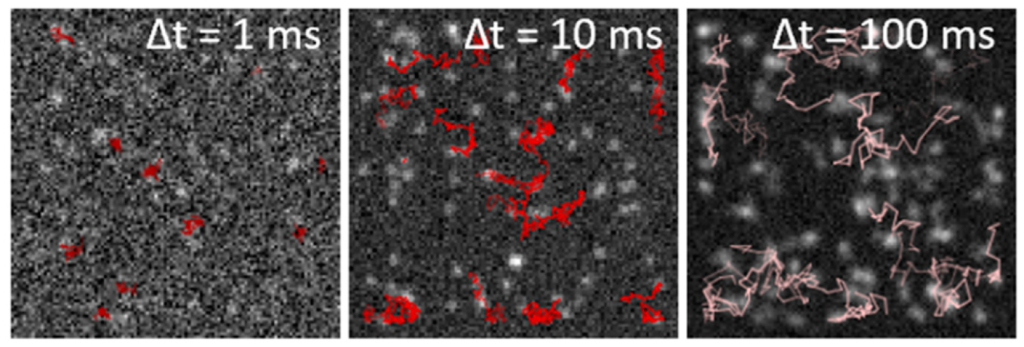
Nanoparticle tracking analysis (NTA) is a method for particle size determination. A well-mixed suspension of nanoparticles is applied into a chamber. Although nanoparticles are smaller than the optical resolution of microscopes, they can be individually detected by the light they scatter. Alternatively, if the nanoparticles are either inherently fluorescent or fluorescently labeled, they can be detected and imaged using a fluorescence microscope (as in Figure 4.1). In either case, images can be collected to track the motion of individual nanoparticles across the microscope stage over time. Given the distance traveled by each particle over a given duration of time, the mean square displacement can be calculated and used to determine the diffusion coefficient. Assuming a spherical particle, the particle size can then be estimated using the Stokes-Einstein equation.
The original version of this chapter contained H5P content. You may want to remove or replace this element.
Exercise 4.1: Diffusion coefficient and mean square displacement
Presume you are conducting NTA analysis on the kaolin nanoparticles from Exercise 3.2 of Chapter 3. The nanoparticles are dispersed in pure water at 22 °C — use the online calculator available from The Engineering ToolBox to determine the dynamic viscosity of water at this temperature. Assume the particles are spherical, and use the number mean diameter (203 nm) for the calculations below. Show your formula and unit conversions/cancellations.
(a) Determine the diffusion coefficient in cm2/s for the nanoparticles.
(b) Determine the mean square displacement in μm2 if the nanoparticles are allowed to diffuse in a 2-dimensional space for a duration of 60 s.
4.2 Sedimentation by gravity and centrifugation
4.2.1 Gravitational sedimentation
Imagine allowing a cup of turbid water containing fine clay particles to sit on a table for an extended duration of time. You might expect to observe some settling or sedimentation of the particles to the bottom of the cup. Sedimentation (or flotation, for particles with a lower density than water) is attributable to the balance of three forces: the gravitational force [latex]\mathbf{{F}_{grav}}}[/latex] due to the gravitational acceleration, the buoyant force [latex]\mathbf{{F}_{buoy}}[/latex] due to displacement of water, and a frictional or drag force [latex]\mathbf{{F}_{drag}}[/latex] between the moving particle and the surrounding fluid (Figure 4.2). The bold text is intended to indicate vectors.
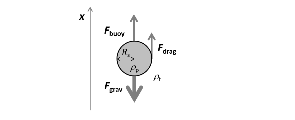
[latex]\mathbf{{F}_{grav}}[/latex] and [latex]\mathbf{{F}_{buoy}}[/latex] are given as Equations 4.7 and 4.8 for a spherical particle with radius [latex]R_{\text{s}}^{3}[/latex] or diameter [latex]d[/latex].
| [latex]\mathbf{{F}_{grav}}=V{{\rho}_{\text{p}}}\mathbf{g}=\frac{4}{3}\pi R_{\text{s}}^{3}{{\rho}_{\text{p}}}\mathbf{g}[/latex] | Gravitational force (4.7) |
| [latex]\mathbf{{F}_{buoy}}=-V{{\rho}_{\text{f}}}\mathbf{g}=-\frac{4}{3}\pi R_{\text{s}}^{3}{{\rho}_{\text{f}}}\mathbf{g}[/latex] | Buoyant force (4.8) |
where [latex]V[/latex] is the volume of the particle, [latex]{\rho}_{\text{p}}[/latex] is the density of the particle, [latex]{\rho}_{\text{f}}[/latex] is the density of the fluid, and [latex]\mathbf{g}[/latex] is the gravitational acceleration vector. If position, [latex]x[/latex], is taken to be positive in the upward direction, then the gravitational acceleration vector will have a negative sign indicating a downward acceleration, i.e., [latex]\mathbf{g}[/latex] = -9.81 m/s2 for the standard gravity of Earth).
The drag force [latex]\mathbf{{F}_{drag}}[/latex] is in the opposing direction of the particle velocity [latex]\mathbf{v}[/latex] and has a magnitude proportional to the friction factor and the particle speed (Equation 4.9):
| [latex]\mathbf{{F}_{drag}}=-f\mathbf{v}=-6\pi\eta {R}_{\text{s}}\mathbf{v}[/latex] | Drag force (4.9) |
Given sufficient time for the gravitational, buoyant, and drag forces to balance (Equation 4.10) and rearranging for velocity after inputting the expressions from Equations 4.7, 4.8, and 4.9 yields the terminal velocity [latex]\mathbf{v_{\infty}}[/latex] (Equation 4.11):
| [latex]0=\mathbf{{F}_{grav}}+\mathbf{{F}_{buoy}}+\mathbf{{F}_{drag}}[/latex] | Force balance (4.10) |
| [latex]\mathbf{v_{\infty}}=\frac{2}{9}\frac{R_{\text{s}}^{2}\left({{\rho}_{\text{p}}}-{{\rho}_{\text{f}}}\right)}{\eta}\mathbf{g}=\frac{{{d}^{2}}\left({{\rho}_{\text{p}}}-{{\rho}_{\text{f}}}\right)}{18\eta}\mathbf{g}[/latex] | Terminal velocity (4.11) |
Hence, if the particle density is higher than the fluid density, the terminal velocity will be in the same direction as the gravitational acceleration vector (i.e., the particle will sink). If the particle density is lower than the fluid density, the terminal velocity will be in the opposite direction as the gravitational acceleration vector (i.e., the particle will float).
The particle- and fluid-related factors before the gravitational acceleration can be grouped as the sedimentation coefficient, [latex]s[/latex], as shown in Equation 4.12:
| [latex]s=\frac{2}{9}\frac{R_{\text{s}}^{2}\left({{\rho}_{\text{p}}}-{{\rho}_{\text{f}}}\right)}{\eta}=\frac{{{d}^{2}}\left({{\rho}_{\text{p}}}-{{\rho}_{\text{f}}}\right)}{18\eta}[/latex] | Sedimentation coefficient (4.12) |
Hence, Equation 4.11 can be expressed in condensed form as Equation 4.13:
| [latex]{\mathbf{{v}_{\infty}}}={s}\mathbf{g}[/latex] | Terminal velocity using the sedimentation coefficient (4.13) |
Interactive Question 4.2: Gravitational sedimentation
The original version of this chapter contained H5P content. You may want to remove or replace this element.
4.2.2 Centrifugal sedimentation
Sedimentation can be a practically useful phenomenon to separate particles from the fluid and dissolved species. The particle “pellet” can be collected as a more concentrated sample or purified by repeated cycles of adding clean solvent and sedimenting the particles, i.e., “washing” the particles. In the quiz above, you should have identified that smaller particles sediment more slowly than large particles. Hence, nanoparticles may settle very slowly, making gravitational sedimentation unfeasible for the separation procedure.
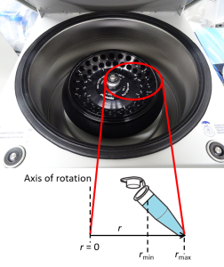
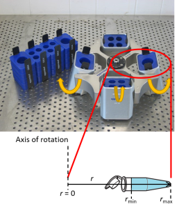
Centrifugation is a common method to accelerate the sedimentation. The spinning chamber inside the centrifuge is called a rotor. The rotor can be placed in either a fixed angle or swinging bucket configuration (Figures 4.3 and 4.4, respectively). In the swinging bucket rotor, each bucket swings outwards during the centrifugation, such that the bottom of each sample holder points radially outwards from the axis of rotation.
The rotation speed of the rotor can be reported as [latex]n[/latex] rotations per minute (rpm) or the angular velocity, [latex]\omega[/latex], per Equation 4.14:
| [latex]\omega =\frac{\left(2\pi\text{ rad/rotation}\right)\left(n\text{ rotations/min}\right)}{60\text{ s/min}}[/latex] | Angular velocity (4.14) |
The inertia of the matter in the rotating device results in a centrifugal “force” outward from the axis of rotation. In a fixed angle rotor, particles in the centrifuge tube will hence travel toward the side of the tube furthest from the axis and overall, “down” the tube due to the placement of the tube at an angle. In a swinging bucket rotor, the buckets swing outward from the axis of rotation (consider swings on a spinning carnival ride), so that the bottom of the centrifuge tube reorients to point directly outward from the axis of rotation while the centrifuge is spinning, resulting in the particles traveling directly “down” the tube.
The centrifugal acceleration, denoted here as [latex]{\mathbf{{g}_{\text{centrifuge}}}}[/latex], increases with the rotational speed as well as the radial distance from the axis of rotation, [latex]r[/latex], following Equation 4.15. It is emphasized that here, [latex]r[/latex] is taken to increase in the outward (downward) direction, such that [latex]{\mathbf{{g}_{\text{centrifuge}}}}[/latex] has a positive value.
| [latex]{\mathbf{{g}_{\text{centrifuge}}}}=r{{\omega }^{2}}[/latex] | Centrifugal acceleration (4.15) |
Comparing this centrifugal acceleration to the gravitational acceleration constant yields the relative centrifugal force (RCF) as Equation 4.16:
| [latex]\text{RCF}=\frac{r{{\omega }^{2}}}{\mathbf{g}}[/latex] | Relative centrifugal force (4.16) |
A common way to denote RCF is as the RCF factor “[latex]{\times}\mathbf{g}[/latex];” for example, centrifuging at an RCF of 500 times the acceleration of gravity can be reported as “[latex]500{\times}\mathbf{g}[/latex]“.
The centrifugal acceleration can be used directly in place of [latex]\mathbf{g}[/latex] in Equation 4.13 to determine the terminal velocity (in the direction outward from the axis of rotation) of a particle in a centrifuge (Equation 4.17):
| [latex]{\mathbf{{v}_{\infty}}}={s}\mathbf{{g}_{\text{centrifuge}}}=s\left(r{{\omega }^{2}}\right)[/latex] | Terminal velocity at a fixed position in a centrifuge (4.17) |
The centrifuge duration required to settle a particle with a given density and size can hence be estimated given the distance to travel (e.g., from the top to the bottom of the fluid column in the centrifuge tube) and the terminal velocity. However, careful consideration of the rotor geometry shown in Figure 4.1 reveals a complication in the calculation of the centrifugal force. As a particle settles from the “top” to the “bottom” of the tube in either the fixed or swinging bucket rotor, it progressively moves further away from the axis of rotation, i.e., the RCF increases over time. To simplify reporting of the RCF, the rotor manufacturer will typically report a table of rotational speed settings (rpm) and the corresponding maximum RCF experienced at the furthest point possible in the rotor (“bottom” of the tube), i.e., the RCFmax. Using the RCFmax value in Equation 4.17 will hence yield the maximum [latex]\mathbf{{v}_{\infty}}[/latex], which overestimates the velocity for particles that initially reside at higher positions in the tube. A more exact evaluation of the centrifuge duration, accounting for the change in [latex]\mathbf{{v}_{\infty}}[/latex] with [latex]{r}[/latex], can be derived upon specifying [latex]\mathbf{{v}_{\infty}}[/latex] as the rate of change in position over time (Equation 4.18):
| [latex]\mathbf{{v}_{\infty}}=\frac{\text{d}r}{\text{d}t}=s\left(r{{\omega}^{2}}\right)[/latex] | Terminal velocity with variable position in a centrifuge (4.18) |
Equation 4.18 is rearranged to Equation 4.19 to separate variables and integrate from position [latex]{{r}_{\text{min}}}[/latex] to [latex]{{r}_{\text{max}}}[/latex] over time 0 to [latex]{t}[/latex], i.e., the time for a particle at the “top” of the tube to settle to the “bottom” of the tube:
| [latex]\int_{0}^{t}{\text{d}t}=\frac{1}{s{{\omega }^{2}}}\int_{{{r}_{\text{min}}}}^{{{r}_{\text{max}}}}{\frac{1}{r}\text{d}r}[/latex] | (4.19) |
Completing the integration results in the following solution (Equation 4.19):
| [latex]t=\frac{1}{s{{\omega }^{2}}}\ln \left( \frac{{{r}_{\text{max}}}}{{{r}_{\text{min}}}} \right)[/latex] | Centrifugation duration required, accounting for variable position (4.20) |
Exercise 4.2: Centrifugation Duration
A sample purification protocol specifies to centrifuge the nanoparticles to “pellet” them at the bottom of a centrifuge tube, so that the water and dissolved species can be removed. An Eppendorf MiniSpin Plus centrifuge is available with a fixed-angle rotor shown in Figure 4.5 below.
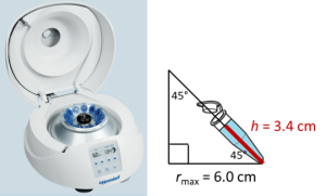
Presume you are centrifuging the kaolin particles from Exercise 3.2 in Chapter 3. Use the number mean diameter (203 nm) and a density of 2600 kg/m3 for kaolin for the centrifugation calculations below.
A volume of 2 mL of the kaolin nanopaticle suspension is added to a centrifuge tube and reaches a height, h, of 3.4 cm in the tube. The product manual specifies a rotor angle of 45° and maximum radius (rmax) of 6 cm, as shown in Figure 4.5. The temperature is 22 °C — use the online calculators available from The Engineering ToolBox to determine the density and dynamic viscosity of water at this temperature. Using trigonometry, determine the minimum radius, rmin, from the center of the rotor to the top of the solution. You set the rotor speed to 5000 rpm.
How long should you centrifuge the particles (in minutes) to pellet the particles from the top to the bottom of the centrifuge tube? Make sure to write all units throughout your calculation and apply any necessary unit conversions to determine the centrifugation time in minutes.
Note on reporting centrifugation settings: Centrifugation settings used in the laboratory are commonly reported as the rotational speed in rpm and duration of centrifugation, along with information on the centrifuge manufacturer. However, as shown in Figures 4.3 and 4.4, the rotor or sample holders inside the centrifuge may be exchangeable for ones with different dimensions or configurations. The specific rotor or sample holder is frequently unreported. Therefore, it is recommmended to report not only the rpm settings but also the RCF (which incorporates information on both the rotational speed and the rotor geometry) to more thoroughly specify the centrifugation method.
4.3 Diffusion and sedimentation equilibrium
Let us revisit our thought experiment on the sample of fine clay particles that has settled by gravity. Close inspection of the bottom of the vial would show that, despite being allowed to settle and equlibrate overnight under stagnant conditions, some particles still reside in the liquid above the deposited sediment, with the turbidity rapidly decreasing away from the bottom of the vessel. Another phenomenon besides gravity sedimentation must be occurring — this phenomenon is diffusion. The combination of diffusion and sedimentation yields a sedimentation equilbrium profile describing the concentration of particles as a function of location.
4.3.1 Fick’s laws of diffusion
Diffusion is an outcome of Brownian motion. First, consider a case where dye molecules (e.g., food coloring) are the solute, and the dye is fully dissolved and mixed in a cup of water to homogenize the dye throughout sample. When the concentration of solute is the same throughout the sample volume, there is no net motion of solute in any particular direction, because the solute molecules are moving randomly in all directions by Brownian motion. In contrast, now consider the case where a concentrated drop of dye solution is added to the sample without mixing. Over time, if diffusion is the only phenomenon at play, the random motion of the molecules will result in the dye showing a net motion away from the high concentration region into the “clean” water until it is ultimately spread evenly throughout the water. This net motion is diffusion.
Fick’s laws of diffusion provide the mathematical representation of this process. Here, we will focus on diffusion in one direction, [latex]x[/latex] through a plane (i.e., 1-dimensional diffusion; for example, “upward” or “downward” in the sample container) (Figure 4.6).
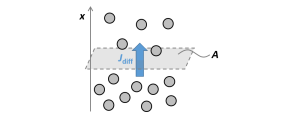
Fick’s first law is given by Equation 4.21:
| [latex]\mathbf{{J}_{\text{diff}}}=-D\frac{\text{d}C}{\text{d}x}[/latex] | Fick’s first law, 1-D diffusive flux (4.21) |
where [latex]\mathbf{J}_{\text{diff}}[/latex] is the net flux of particles or molecules across the plane (units of moles length-2 time-1), [latex]D[/latex] is the diffusion coefficient as before (units of length2 time-1), and [latex]C[/latex] is the molar concentration (units of moles length-3) at position [latex]x[/latex]. [latex]{\text{d}C\text{/d}x}[/latex] is the concentration gradient across the plane. The minus sign indicates the directionality of the net diffusion from high to low concentration, i.e., “down” the concentration gradient. If the concentration decreases as [latex]x[/latex] increases, then [latex]{\text{d}C\text{/d}x}[/latex] is negative and the net flux, [latex]\mathbf{{J}_{\text{diff}}}[/latex], will then have a positive value, indicating net motion in the [latex]+x[/latex] direction. For the well-mixed case, the concentration gradient, [latex]{\text{d}C\text{/d}x}[/latex], is zero, and hence there will be zero net flux.
Given the cross-sectional area, [latex]A[/latex], through which the flux is occurring, the net rate of particles of molecules crossing the plane is [latex]\mathbf{{J}_{\text{diff}}}{A}[/latex] (units of moles time-1). The mass flux or the mass transfer rate can be determined by multiplying the molar flux units by the molar mass of the particle (i.e., [latex]{\rho}_{\text{p}}\left({4/3}\right)\pi R_{\text{s}}^{3}{N}_{\text{A}}[/latex] for spherical particles with radius [latex]R_{\text{s}}[/latex] and density [latex]{\rho}_{\text{p}}[/latex], where [latex]{N}_{\text{A}}[/latex] is Avogadro’s number) or the molar mass of the molecule for a dissolved solute. Alternatively, if [latex]C[/latex] is specified as a mass concentration instead of a molar concentration for Equation 4.21, then the units for [latex]\mathbf{{J}_{\text{diff}}}[/latex] will directly be mass length-2 time-1.
The quiz in Interactive Question 4.3 below will test your knowledge on interpreting Fick’s first law for different scenarios.
Interactive Question 4.3: Diffusion
When answering this quiz, it is recommended to have a pen and paper on hand to write and combine relevant equations given throughout this chapter indicating the relationships between the diffusion coefficient, flux, particle size, and molar versus mass concentration units.
The original version of this chapter contained H5P content. You may want to remove or replace this element.
Fick’s first law provides the flux at one given location and time point. However, if there is net transfer, the concentrations will change over time, also resulting in a changing net flux rate, until a steady-state is reached (i.e., no net change over time). If one wanted to track the change in concentration over time [latex]t[/latex], then Fick’s second law will be required (Equation 4.22):
| [latex]\frac{\partial C}{\partial t}=D\frac{{{\partial }^{2}}C}{\partial {{x}^{2}}}[/latex] | Fick’s second law, 1-D diffusion (4.22) |
However, the remainder of this course book will focus only on steady-state results, so Fick’s second law will not be revisited.
4.3.2 Sedimentation equilibrium
Let us reconsider again the clay particles in the vial and the processes covered in this chapter. If the particles are denser than water and only experienced gravitation sedimentation, then we would expect every particle to eventually deposit on the bottom surface of the vial. On the other hand, if the particles only experienced Brownian motion and diffusion without sedimentation, we would expect them to move away from any regions of higher concentration (e.g., the bottom of the vial) and distribute homogeneously. In reality, the combined influence of both processes results in the concentration profile to be achieved at equilbrium (Figure 4.7).
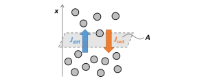
The sedimentation equilbrium profile can be theoretically derived by determining the conditions at which the net flux is zero. This steady-state condition or flux balance is expressed as Equation 4.23. With vector notation, taking x increasing in the upward direction and assuming the particle is denser than water, [latex]\mathbf{{J}_{\text{sed}}}[/latex] will be negative, and [latex]\mathbf{{J}_{\text{diff}}}[/latex] will be positive.
| [latex]0=\mathbf{{J}_{\text{sed}}}+\mathbf{{J}_{\text{diff}}}[/latex] | Flux balance (4.23) |
The sedimentation flux [latex]\mathbf{J_{sed}}[/latex] at position [latex]x[/latex] can be computed as the product of the terminal sedimentation velocity [latex]\mathbf{v_{\text{\infty}}}[/latex] and the concentration [latex]C[/latex] at position [latex]x[/latex] (Equation 4.24), resulting in flux units of moles length-2 time-1 for [latex]C[/latex] in molar concentration units, or mass length-2 time-1 for [latex]C[/latex] in mass concentration units:
| [latex]\mathbf{{J}_{sed}}=\mathbf{{v}_{\infty}}{C}[/latex] | Sedimentation flux (4.24) |
Inputting Equations 4.21 and 4.24 into Equation 4.23 then yields Equation 4.25:
| [latex]\mathbf{{v}_{\infty}}{C}=D\frac{\text{d}C}{\text{d}x}[/latex] | (4.25) |
For sedimentation equilibrium under gravity, the terminal velocity is [latex]s\mathbf{g}[/latex]. The steady-state concentration [latex]C[/latex] as a function of location [latex]x[/latex] can then be solved per Equations 4.26 to 4.29:
| [latex]s\mathbf{g}C=D\frac{\text{d}C}{\text{d}x}[/latex] | (4.26) |
| [latex]\int_{{C}_{0}}^{{C\left({x}\right)}}{\frac{1}{C}\text{d}C}=\int_{{x}_{0}}^{x}{\frac{s\mathbf{g}}{D}\text{d}x}[/latex] | (4.27) |
| [latex]\ln\left(\frac{{C}\left({x}\right)}{{C}_{0}}\right)=\frac{s\mathbf{g}}{D}\left(x-0\right)[/latex] | (4.28) |
| [latex]{C}\left({x}\right)={{C}_{0}}{{\operatorname{e}}^{\frac{s\mathbf{g}}{D}{x}}[/latex] | Sedimentation equilibrium profile under gravity (4.29) |
where [latex]C_{0}[/latex] is the concentration at [latex]x = 0[/latex]. It is emphasized again that [latex]\mathbf{g}[/latex] is a negative value when taking [latex]x[/latex] to increase in the upward direction. Hence, the concentration should decrease exponentially from the bottom of the container for sedimentation equilibrium under gravity.
For sedimentation in a centrifuge, the scenario is slightly more complicated because the centrifugal force increases with position [latex]r[/latex] from the axis of rotation (Equation 4.30). The integrated solution is provided in Equation 4.31 for sedimentation equilibrium in a centrifuge.
| [latex]s\left({{\omega }^{2}}r\right)C=D\frac{\text{d}C}{\text{d}r}[/latex] | (4.30) |
| [latex]{C\left({r}\right)}={{C}_{0}}{{\operatorname{e}}^{\frac{s{{\omega }^{2}}}{2D}{{r}^{2}}}}[/latex] | Sedimentation equilibrium profile in a centrifuge (4.31) |
It is noted that because [latex]r[/latex] is taken to be positive in the outward direction, Equation 4.31 indicates that the concentration further “down” the tube will be higher than the concentration further “up” the tube, as expected. The distance dependence of the sedimentation equilibrum profile in the centrifuge is more significant compared to the sedimentation equilibrium profile under gravity.
Let us conclude by considering the impact of particle size and other key factors in the sedimentation equilibrium. A larger or denser particle will have a higher sedimentation coefficient [latex]s[/latex]. Larger particles also have a smaller diffusion coefficient [latex]D[/latex]. These terms appear together as [latex]s/D[/latex] in the exponential term. Hence, the concentration of very large, high density particles will drop off extremely rapidly away from the bottom of the vial. On the other hand, the presence of small, lower density particles will extend further into the liquid above the sediment deposit. For nanoscale molecules (e.g., proteins) or nanoparticles that have high diffusion coefficients, the exponential term will be close to e0, i.e., 1, and the sample can remain well-dispersed and nearly homogeneous for long durations of time. Higher temperature also results in a higher diffusion coefficient. Finally, the solvent viscosity cancels in the [latex]s/D[/latex] term for spherical particles and hence should have no effect on the sedimentation equilibrium.