
4
3.1 Terminology standards defining nanomaterials
Chapter 1 provided a brief definition of a nanomaterial as any material having one or more dimensions in the size range of 1 nm to 100 nm. The selection of these specific bounds for the size limits may appear somewhat arbitrary. For example, in the emerging field of microplastics and nanoplastics, some debate exists regarding whether the upper size limit should be set at 100 nm or 1000 nm (Gigault et al., Environ. Pollut. 2018, 235, 1030-1034). Here, a terminology standard is useful to encourage consistent use of the same definition across a wide audience (e.g., resesarchers, commercial suppliers or vendors, and regulatory agencies). The terminology standard can also delve into further nuances of the definition of nanomaterials, as well as other related terminology.
Exercise 3.1: Terminology standards for nanotechnology
Review the following two documentary standards related to definitions of nanomaterials:
- ASTM E2456-06(2020) — Standard Terminology Relating to Nanotechnology
- ISO 80004-1:2023(en) — Nanotechnologies – Vocabulary — Part 1: Core vocabulary
It is noted that ASTM standards may be freely accessible at institutions with an ASTM COMPASS subscription. At the time of this writing, the text of ISO 80004-1:2023(en) is accessible from the ISO catalog page linked above by selecting “Read Sample.”
1. How is a “nanomaterial” defined in each standard?
2. Read the definitions for “transitive” and “non-transitive” in the ASTM standard, as well as “nanoscale phenomenon” in the ISO standard. Is it required for a nanomaterial to exhibit a “transitive” property or “nanoscale phenomenon” to meet the definition of a nanomaterial?
3. What is the definition of a “primary particle,” an “agglomerate,” and an “aggregate”? Test your knowledge on this concept using Interactive Question 3.2 at the end of this chapter.
3.2 Overview of nanoparticle size measurements and electron microscopy
Given that nanomaterials are defined based on a size criterion (at least one dimension in the range of 1 nm to 100 nm), size is arguably the most important property of a nanomaterial. As discussed in Chapter 1 and Section 3.1 above, size can also be a crucial factor in enabling unique properties of nanomaterials, such as their optical or electronic behavior, or enhancing other behaviors, such as chemical reactivity or transport and delivery of the nanomaterials in a desired application. The remainder of this chapter focuses on measures of size and size distributions. Primary focus is placed on individually dispersed, spherical nanoparticles. Finally, a brief discussion of measures of shape and aggregate or agglomerate morphology is then provided.
Nanoparticle sizes or size distributions can be evaluated using a variety of analytical approaches, including the following:
- Imaging methods, e.g., transmission electron microscopy (TEM) and scanning electron microscopy (SEM)
- Optical spectroscopy, e.g., ultraviolet (UV)-visible spectroscopy
- Light scattering, e.g., static light scattering (SLS) and dynamic light scattering (DLS)
- Size separations, e.g., filtration, centrifugation, and field flow fractionation (FFF) — coupled with detection or quantification methods to evaluate the size fractions
- Mass-based analyses, e.g., single particle inductively coupled plasma mass spectrometry (spICPMS)
- Other methods not be discussed in depth here include atomic force microscopy (AFM), nanoparticle tracking analysis (NTA), and electrospray differential mobility analysis (ES-DMA)
Imaging methods, i.e., electron microscopy, are briefly covered here, and data collected using imaging methods are utilized for the data analysis examples in this chapter. Principles and data analyses for several of the other \classes of methods will be explored in depth in the laboratories presented late in this course book (UV-vis spectroscopy, DLS, FFF, and spICPMS). It is noted that different methods that operate on different principles may yield results that differ quantitatively. When the same property (e.g., size) is measured on the same sample using methods based on different principles, the various measurements are considered to be “orthogonal” (see note below). With a firm understanding of the principles of the measurements and the different biases or uncertainties associated with each type of measurement, one can interpret all of the measurements in a coherent manner to gain a more comprehensive understanding of the sample.
Note on “orthogonal” versus “complementary” measurements: Following the NIST publication, “Orthogonal Measurements,” orthogonal measurements are considered a subset of complementary measurements. Measurements that are complementary but not orthogonal include the following cases: (i) the same property is measured on the same sample using methods that operate on the same principle; (ii) different properties are measured on the same sample; (iii) measurements are collected for the same purpose but comparing different samples.
Imaging methods are valuable tools because they provide a visual representation of the sample, allowing facile evaluation of features such as particle shape, along with determination of the sizes of individual nanoparticles within a population. However, sample preparation can become challenging, as samples are most commonly deposited and dried onto a substrate for analysis. During the image analysis, it may then be difficult to determine whether clusters of nanoparticles that appear in the images were already present as aggregates or agglomerates in the original sample or whether they had formed only during the sample deposition.
Typical optical microscopes using visible light and lenses are generally not suitable for imaging nanoparticles because the resolution (which corresponds the smallest size features that can be distinguished across the image) is directly limited to approximately half the wavelength (λ) of electromagnetic radiation used. Visible light sources used for optical microscopy produce light in the 400 nm to 700 nm wavelength range. Hence, the theoretical resolution limit is approximately 200 nm, with a larger practical limit when considering the design and manufacturing of the optics. A nanoparticle with sizes between 1 nm to 100 nm would not be resolvable in an optical microsope.
Electron microscopes utilize high energy electrons for imaging, with λ ∝ V -1/2, where V is the energy applied in the electron microscope. Electron microscopy can be conducted in transmission or scanning electron microscopy modes (TEM or SEM, respectively). In TEM, the sample is situated directly in between the electron source and the camera. Materials dense enough to block the transmission of electrons through the sample to the camera appear as dark regions in the image on a bright background. In SEM, the camera is placed at an angle and observes electrons that are scattered by materials in the sample. These scattered electrons appear as bright regions in the image on a dark background.
Because of the high energy (small wavelength) used in electron microscopy, extremely small objects can be resolved. A 300 kiloelectronvolt (keV) TEM instrument has a theoretical resolution of approximately 2 picometers (pm), i.e., 0.002 nm, with a practical limit of approximately 0.1 nm to 0.3 nm (JEOL, 2025). SEM typically has coarser resolution than TEM, with limits of approximately 0.5 nm to 4 nm (JEOL, 2025)
Other resources: For a more thorough description of TEM and SEM, along with diagrams of the instrument setup, the reader is recommended to visit the following pages hosted on the Microbe Notes website:
- Mokobi, F. Transmission Electron Microscope (TEM)- Definition, Principle, Images, Microbe Notes, 2022, https://microbenotes.com/transmission-electron-microscope-tem/
- Mokobi, F. Scanning Electron Microscope (SEM): Principle, Parts, Uses, Microbe Notes, 2024, https://microbenotes.com/scanning-electron-microscope-sem/
Interactive Question 3.1
The following image shows electron micrographs presented in the NIST Report of Investigation for Reference Material® 8012 — Gold Nanoparticles, Nominal 30 nm Diameter (NIST, 2015). Based on the principles of TEM and SEM, drag the label onto the image that was collected using each method.
The original version of this chapter contained H5P content. You may want to remove or replace this element.
3.3 Measures of size distributions and mean diameters for spherical particles
Close inspection of the electron micrographs above for NIST SRM 8012 (Gold Nanoparticles, Nominal 30 nm Diameter) reveals that each particle has a slightly different size; that is, there is no single size value representing every nanoparticle in the population, but rather a size distribution. A more dramatic demonstration of polydispersity, i.e., a wide size distribution, is shown in Figure 3.1 for a polydisperse sample of nanoscale to colloidal lignin particles that undergo size stratification when dried under controlled conditions onto a substrate. The sample as a whole is highly polydisperse, while each layer comprises a more monodisperse subset of the population.
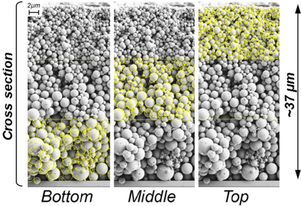
Size distributions can be communicated as a histogram showing the frequency or percent of nanoparticles residing in various size bins, or a mean and variance representing the average size across the population and degree of polydispersity in the sizes, respectively. Different measurement techniques or data analyses will yield different forms of the “average” size. Specifically, sizes in the distribution can be weighted by number — i.e., each individual particle size is considered equally in the averaging — or some other feature such as area or mass, wherein larger particles are weighted more heavily, biasing the average size to a larger value. The documentary standard ASTM E2578-07(2022) — Standard Practice for Calculation of Mean Sizes/Diameters and Standard Deviations of Particle Size Distributions, provides a systematic definition of 22 different “mean” diameters. Seven of these mean diameters, along with computation of the variance and standard deviation, are highlighted here.
3.3.1 Number (arithmetic) mean diameter and variance
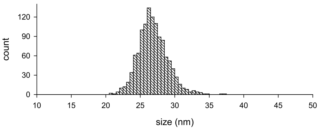
Imaging analyses have the advantage of being able to determine individual nanoparticle sizes in the micrograph. In general, given the instrument calibration to apply a scale bar to the image, an image analysis software can be utilized to outline each particle, determine the image area (pixels) covered by each particle, and convert the image area to an equivalent spherical diameter for each particle. Measurements taken on an ensemble of many (e.g. thousands of) nanoparticles can be used to generate a histogram showing a count of the number of particles in each size bin. An example histogram is provided in Figure 3.2 for the SEM analysis of a total of 1185 gold nanoparticles, as reported in the NIST Report of Investigation for SRM 8012 (Gold Nanoparticles, Nominal 30 nm Diameter). Other methods capable of producing a data set with individual particle sizes include spICPMS and NTA.
Given the sizes of each nanoparticle in the distribution, the number (arithmetic) mean diameter, [latex]\overline{{{d}_{\text{n}}}}[/latex], and sample variance, [latex]\sigma^{2}[/latex], are computed using Equations 3.1 and 3.2, respectively,
| [latex]\overline{{d}_{\text{n}}}=\frac{\sum\limits_{i}{\left( {{n}_{i}}{{d}_{i}} \right)}}{N}=\sum\limits_{i}{\left({{f}_{\text{n},i}}{{d}_{i}} \right)}[/latex] | (3.1) |
| [latex]\sigma^{2} =\frac{\sum\limits_{i}{\left[ {{n}_{i}}{{\left( {{d}_{i}}-\overline{{d}_{n}} \right)}^{2}} \right]}}{N-1}[/latex] | (3.2) |
where [latex]{d}_{i}[/latex] is the mean size associated with each size bin, [latex]{i}[/latex]; [latex]{n}_{i}[/latex] is the number of particles in bin [latex]{i}[/latex]; [latex]{N}[/latex] is the total number of particles in the data set; and [latex]{f}_{\text{n},i}[/latex] is the number fraction of particles in bin [latex]{i}[/latex], i.e., [latex]{f}_{\text{n},i}}={{{n}_{i}}}/{N}[/latex]. The standard deviation, [latex]\sigma[/latex], is the square root of the variance.
3.3.2 Mean area diameter and mean volume (or mass) diameter
Larger particles represent disproportionately more of the total surface area and total volume (or mass, where mass is proportional to particle volume by the density) occupied within the sample, than an equivalent number of small particles — this fact can be visually apparent in Figure 3.1, in which many small particles would be needed to occupy the same amount of space in the image as the largest particle. Two approaches can be taken to account for the weighting of the mean size for area or volume.
The first approach is to compute the mean surface area or the mean volume across all the particles, and then calculate the spherical particle diameter corresponding to that mean area or volume, respectively. This approach yields the “mean surface (area) diameter” or “mean volume diameter,” following the terminology assigned in ASTM E2578-07(2022). The calculation is shown in full for the mean surface (area) diamter. First, the surface area, A, for a spherical particle of diameter d is noted (Equation 3.3). The mean surface area, [latex]\overline{A}[/latex], is computed as the total surface area for all particles and dividing by the number of particles (Equation 3.4), which can further be condensed using the definition above for [latex]{f}_{\text{n},i}}[/latex]. Finally, a “mean surface” diameter is calculated that would result in this mean surface area (Equation 3.5).
| [latex]A=\pi {{d}^{2}}[/latex] | (3.3) |
| [latex]\overline{A}=\frac{\sum\limits_{i}{\left( {{n}_{i}}\times \pi d_{i}^{2} \right)}}{N}=\pi \sum\limits_{i}{\left( {{f}_{\text{n},i}}d_{i}^{2} \right)}[/latex] | (3.4) |
| [latex]\overline{{d}_{s}}={{\left( \frac{\overline{A}}{\pi } \right)}^{1/2}}={{\left[ \frac{\sum\limits_{i}{\left( {{n}_{i}}d_{i}^{2} \right)}}{N} \right]}^{1/2}}={{\left[ \sum\limits_{i}{\left( {{f}_{\text{n},i}}d_{i}^{2} \right)} \right]}^{1/2}}[/latex] | (3.5) |
A similar approach can be taken to compute the mean volume diameter, [latex]\overline{{{d}_{\text{v}}}}[/latex] (Equation 3.6):
| [latex]\overline{{d}_{\text{v}}}={{\left[ \frac{\sum\limits_{i}{\left( {{n}_{i}}d_{i}^{3} \right)}}{N} \right]}^{1/3}}={{\left[ \sum\limits_{i}{\left( {{f}_{\text{n},i}} d_{i}^{3} \right)} \right]}^{1/3}}[/latex] | (3.6) |
3.3.3 Diameter-weighted, area-weighted, and volume- (or mass-) weighted mean diameter
An alternative approach can be applied for weighting the particle sizes and may be required when particle sizes are not able to measured on individual nanoparticles. Consider a scenario in which a dry particle sample is sieved through sequentially smaller mesh sizes, with the material collected on each sieve representing a size bin; thereafter, the quantity of particles in each bin is measured not by counting but rather by weighing the mass of particles in each bin, [latex]{\text{m},i}[/latex], on a balance. In this scenario, the most straightforward approach to “average” the size would be to weight each bin diameter by its measured mass fraction, [latex]{f}_{\text{m},i}[/latex], rather than number of particles (Equation 3.7), which is denoted here as [latex]\overline{{d}_{\text{v-w}}}[/latex] or [latex]\overline{{d}_{\text{m-w}}}[/latex] for “volume-weighted” or “mass-weighted,” respectively:
| [latex]\overline{{d}_{\text{v-w}}}=\overline{{d}_{\text{m-w}}}=\frac{\sum\limits_{i}{\left( {{m}_{i}}{{d}_{i}} \right)}}{\sum\limits_{i}{\left( {{m}_{i}} \right)}}=\sum\limits_{i}{\left( {{f}_{\text{m},i}}{{d}_{i}} \right)}[/latex] | (3.7) |
Taking each particle bin to be completely monodisperse and expanding the particle mass as density times volume, Equation 3.7 can also be represented as Equation 3.8 to reintroduce the number of particles per bin, [latex]{\text{n},i}[/latex], that would yield the measured mass:
| [latex]\overline{{d}_{\text{v-w}}}=\overline{{d}_{\text{m-w}}}=\frac{\sum\limits_{i}{\left[ {{n}_{i}}\left( \rho \frac{\pi }{6}d_{i}^{3} \right){{d}_{i}} \right]}}{\sum\limits_{i}{\left[ {{n}_{i}}\left( \rho \frac{\pi }{6}d_{i}^{3} \right) \right]}}=\frac{\sum\limits_{i}{\left[ {{n}_{i}}d_{i}^{4} \right]}}{\sum\limits_{i}{\left[ {{n}_{i}}d_{i}^{3} \right]}}[/latex] | (3.8) |
This computation for [latex]\overline{{d}_{\text{m-w}}}[/latex] is equivalent to that specified for the “volume-weighted mean diameter” in ASTM E2578-07(2022).
Similarly, the diameter-weighted and surface area-weighted mean diameters can be computed as Equations 3.9 and 3.10, respectively:
| [latex]\overline{{d}_{\text{d-w}}}=\frac{\sum\limits_{i}{\left[ {{n}_{i}}d_{i}^{2} \right]}}{\sum\limits_{i}{\left[ {{n}_{i}}d_{i} \right]}}[/latex] | (3.9) |
| [latex]\overline{{d}_{\text{s-w}}}=\frac{\sum\limits_{i}{\left[ {{n}_{i}}d_{i}^{3} \right]}}{\sum\limits_{i}{\left[ {{n}_{i}}d_{i}^{2} \right]}}[/latex] | (3.10) |
3.3.4 Geometric mean diameter
The last type of mean diameter that will be covered is the geometric mean diameter. This mean is relevant because particle populations commonly show a lognormal size distribution, rather than a normal or Gaussian distribution. That is, the distribution becomes a nomal distribution when the logarithm of the size is used as the measurand; hence, size distributions are frequently plotted on a semi-log plot. For a lognormal distribution, the arithmetic mean will not coincide with the mode of the distribution but rather a larger value. On the other hand, if the arithmetic mean is computed on the logarithm of the size (then converted using the antilog) as per Equation 3.11, this “gemetric mean diameter,” [latex]\overline{{{d}_{\text{g}}}}[/latex], will coincide with the mode of the size distribution:
| [latex]\overline{{{d}_{\text{g}}}}=\exp \left[ \frac{\sum\limits_{i}{\left( {{n}_{i}}\ln {{d}_{i}} \right)}}{{{N}_{i}}} \right][/latex] | (3.11) |
Exercise 3.2: Example computation of various mean diameters
The data from the histogram shown in Figure 3.2 for NIST SRM 8012 (Gold Nanoparticles, Nominal 30 nm Diameter) are provided in Table 3.1 below, along with computations the arithmetic (number) mean diameter, variance and standard deviation, mean surface diameter, mean volume diameter, volume- (or mass-) weighted mean diameter, and geometric mean diameter.
Table 3.1. Data for the histogram in Figure 3.2 and calculations of various mean diameters (click to reveal):
| Bin, i | [latex]{d}_{i}[/latex] (nm) | [latex]{n}_{i}[/latex] | [latex]{f}_{i}[/latex] | [latex]{{n}_{i}}{{d}_{i}}[/latex] (nm) | [latex]{{n}_{i}}{{\left( {{d}_{i}}-\overline{{d}_{n}} \right)}^{2}}[/latex] (nm2) | [latex]{{n}_{i}}d_{i}^{2}[/latex] (nm2) | [latex]{{n}_{i}}d_{i}^{3}[/latex] (nm3) | [latex]{{n}_{i}}d_{i}^{4}[/latex] (nm4) | [latex]{{n}_{i}}\ln {{d}_{i}}[/latex] |
| 1 | 20.25 | 0 | 0.0000 | 0 | 0 | 0 | 0 | 0 | 0 |
| 2 | 20.75 | 2 | 0.0017 | 42 | 74 | 861 | 17868 | 370768 | 6 |
| 3 | 21.25 | 1 | 0.0008 | 21 | 31 | 452 | 9596 | 203909 | 3 |
| 4 | 21.75 | 4 | 0.0034 | 87 | 104 | 1892 | 41156 | 895153 | 12 |
| 5 | 22.25 | 10 | 0.0084 | 223 | 211 | 4951 | 110151 | 2450869 | 31 |
| 6 | 22.75 | 12 | 0.0101 | 273 | 201 | 6211 | 141295 | 3214451 | 37 |
| 7 | 23.25 | 19 | 0.0160 | 442 | 246 | 10271 | 238793 | 5551949 | 60 |
| 8 | 23.75 | 34 | 0.0287 | 808 | 326 | 19178 | 455480 | 10817661 | 108 |
| 9 | 24.25 | 61 | 0.0515 | 1479 | 411 | 35872 | 869891 | 21094868 | 194 |
| 10 | 24.75 | 64 | 0.0540 | 1584 | 281 | 39204 | 970299 | 24014900 | 205 |
| 11 | 25.25 | 100 | 0.0844 | 2525 | 255 | 63756 | 1609845 | 40648594 | 323 |
| 12 | 25.75 | 109 | 0.0920 | 2807 | 131 | 72274 | 1861051 | 47922055 | 354 |
| 13 | 26.25 | 134 | 0.1131 | 3518 | 48 | 92334 | 2423777 | 63624155 | 438 |
| 14 | 26.75 | 120 | 0.1013 | 3210 | 1 | 85868 | 2296956 | 61443563 | 394 |
| 15 | 27.25 | 110 | 0.0928 | 2998 | 18 | 81682 | 2225831 | 60653897 | 364 |
| 16 | 27.75 | 89 | 0.0751 | 2470 | 73 | 68536 | 1901862 | 52776667 | 296 |
| 17 | 28.25 | 84 | 0.0709 | 2373 | 165 | 67037 | 1893802 | 53499915 | 281 |
| 18 | 28.75 | 58 | 0.0489 | 1668 | 210 | 47941 | 1378293 | 39625923 | 195 |
| 19 | 29.25 | 52 | 0.0439 | 1521 | 300 | 44489 | 1301311 | 38063334 | 176 |
| 20 | 29.75 | 40 | 0.0338 | 1190 | 337 | 35403 | 1053224 | 31333425 | 136 |
| 21 | 30.25 | 27 | 0.0228 | 817 | 313 | 24707 | 747377 | 22608163 | 92 |
| 22 | 30.75 | 16 | 0.0135 | 492 | 244 | 15129 | 465217 | 14305415 | 55 |
| 23 | 31.25 | 10 | 0.0084 | 313 | 194 | 9766 | 305176 | 9536743 | 34 |
| 24 | 31.75 | 8 | 0.0068 | 254 | 192 | 8065 | 256048 | 8129520 | 28 |
| 25 | 32.25 | 4 | 0.0034 | 129 | 117 | 4160 | 134168 | 4326920 | 14 |
| 26 | 32.75 | 6 | 0.0051 | 197 | 209 | 6435 | 210759 | 6902342 | 21 |
| 27 | 33.25 | 4 | 0.0034 | 133 | 164 | 4422 | 147040 | 4889074 | 14 |
| 28 | 33.75 | 3 | 0.0025 | 101 | 143 | 3417 | 115330 | 3892390 | 11 |
| 29 | 34.25 | 1 | 0.0008 | 34 | 55 | 1173 | 40177 | 1376076 | 4 |
| 30 | 34.75 | 1 | 0.0008 | 35 | 62 | 1208 | 41963 | 1458207 | 4 |
| 31 | 35.25 | 0 | 0.0000 | 0 | 0 | 0 | 0 | 0 | 0 |
| 32 | 35.75 | 0 | 0.0000 | 0 | 0 | 0 | 0 | 0 | 0 |
| 33 | 36.25 | 0 | 0.0000 | 0 | 0 | 0 | 0 | 0 | 0 |
| 34 | 36.75 | 1 | 0.0008 | 37 | 98 | 1351 | 49633 | 1824019 | 4 |
| 35 | 37.25 | 1 | 0.0008 | 37 | 108 | 1388 | 51687 | 1925330 | 4 |
| Sum of column: | N = 1185 | 1 | 31814 | 5324 | 859430 | 23365057 | 639380254 | 3895 | |
| Variance: |
[latex]\sigma^{2}[/latex] = 4.5 nm | ||||||||
| Mean diameters and standard deviation: | [latex]\overline{{d}_{\text{n}}}[/latex] = 26.8 nm | [latex]\sigma[/latex] = 2.1 nm | [latex]\overline{{d}_{\text{s}}}[/latex] = 26.9 nm | [latex]\overline{{d}_{\text{v}}}[/latex] = 27.0 nm | [latex]\overline{{d}_{\text{v-w}}}[/latex] = 27.4 nm | [latex]\overline{{{d}_{\text{g}}}}[/latex] = 26.8 nm | |||
The results for the mean sizes show and increasing trend from number to surface to volume mean diameter. In addition, the volume-weighted mean diameter is larger than the volume mean diameter. However, these means are all similar (within 1 nm). Note that the SRM 8012 nanoparticles used for this example showed a low degree of polydispersity (Figure 3.2).
Download the linked practice spreadsheet for the above data set (without calculations), along with a second data set for kaolin clay particles in the colloidal size range with the distribution shown in Figure 3.3.
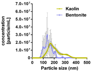
1. Compute [latex]\overline{{d}_{\text{n}}}[/latex] and [latex]\sigma[/latex]. Based on the standard deviation, is the kaolin sample more or less polydisperse than the SRM 8012 gold nanoparticle sample?
2. Compute [latex]\overline{{d}_{\text{s}}}[/latex], [latex]\overline{{d}_{\text{v}}}[/latex], [latex]\overline{{d}_{\text{v-w}}}[/latex], and [latex]\overline{{d}_{\text{g}}}[/latex] for the kaolin particles.
(a) Is the trend in the different sizes the same as that observed for the gold nanoparticles?
(b) Is there greater or lesser distinction between the different mean sizes for the kaolin particles or the gold nanoparticles?
3.4 Measures of size for non-spherical particles or structured particles
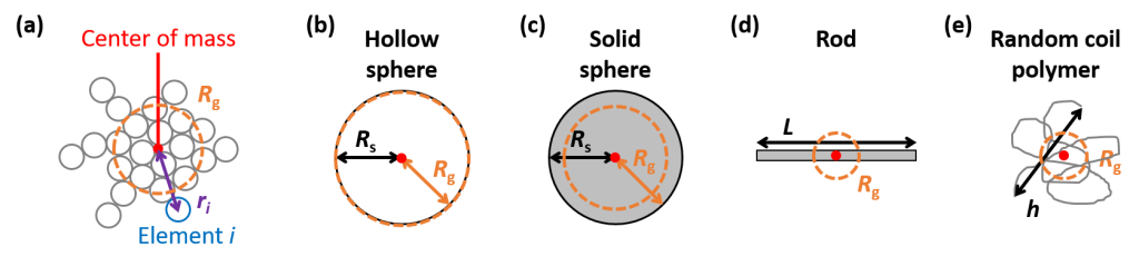
Sizes for non-spherical particles or structured particles — e.g., core-shell particles or a liposomal particle with a shell encapsulating a liquid interior — are more challenging to describe. In these cases, radius of gyration ([latex]{R}_{\text{g}}[/latex]) can be a useful measure that is flexible to accommodate any shape or structure of particle. The radius of gyration represents the root mean square distance of the matter comprising the particle from the center of mass and is closely related to the inertia of the particle. Figure 3.4(a) shows a schematic of a rigid assemblage of mass elements, [latex]{i}[/latex], comprising an object. The moment of inertia for each element, [latex]{I}_{i}[/latex], is calculated as [latex]{m}_{i}{r}_{i}^{2}[/latex], where [latex]{m}_{i}[/latex] is the mass of the element and [latex]{r}_{i}[/latex] is its distance from the center of mass.
The radius of gyration, [latex]{R}_{\text{g}}[/latex], is computed as Equation 3.12:
| [latex]{{R}_{\text{g}}}=\sqrt{\frac{\sum\limits_{i}{\left( {{m}_{i}}r_{i}^{2} \right)}}{\sum\limits_{i}{\left( {{m}_{i}} \right)}}}[/latex] | (3.12) |
The relationships between [latex]{R}_{\text{g}}[/latex] and other size measures for particles with relatively simple shapes and structures are provided in Equations 3.13 to 3.16 for a hollow sphere with radius [latex]{R}_{\text{s}}[/latex] (infinitely thin shell) (Figure 3.4(b)), solid sphere with outer radius [latex]{R}_{\text{s}}[/latex] (Figure 3.4(c)), rod with length [latex]{L}[/latex] (infinitely thin) (Figure 3.4(d)), and random coil polymer with end-to-end chain distance [latex]{h}[/latex] (Figure 3.4(e)) (it is noted that [latex]{h}^{2}[/latex] is proportional to the molecular weight of the polymer).
| [latex]{{R}_{\text{g}}}={{R}_{\text{s}}}[/latex] | Hollow sphere (3.13) |
| [latex]{{R}_{\text{g}}}=\sqrt{\frac{3}{5}}{{R}_{\text{s}}}[/latex] | Solid sphere (3.14) |
| [latex]{{R}_{\text{g}}}=\frac{L}{\sqrt{12}}[/latex] | Rod (3.15) |
| [latex]{{R}_{\text{g}}}=\frac{h}{\sqrt{6}}[/latex] | Random coil polymer (3.16) |
Considering the above relationships, combining measurements on the physical (outer) size of the particle and radius of gyration can be useful to evaluate structural characteristics of the particle that otherwise might not be visible or easily apparent, for example, whether a spherical particle is hollow or filled. An elegant demonstration of this analysis has been presented for distinguishing empty versus filled liposome nanoparticles for drug delivery (Some, n.d.).
3.5 Measures of aggregate or agglomerate structure
When multiple particles attach to form an aggregate or agglomerate, they may form either a dense or loose structure, which can be described quantitatively by the fractal dimension, [latex]{D}_{\text{f}}[/latex]. The fractal dimension can be determined via the following process (Figure 3.5(a)): (i) identify the center of mass of the object (i.e., the aggregate or agglomerate structure); (ii) imagine concentric spheres of increasing radius [latex]{r}[/latex] around the center of mass; (iii) determine the portion of the mass of the object, [latex]{m}_{r}[/latex], contained within each radius [latex]{r}[/latex]; and (iv) determine the relationship between [latex]{m}_{r}[/latex] and [latex]{r}[/latex].
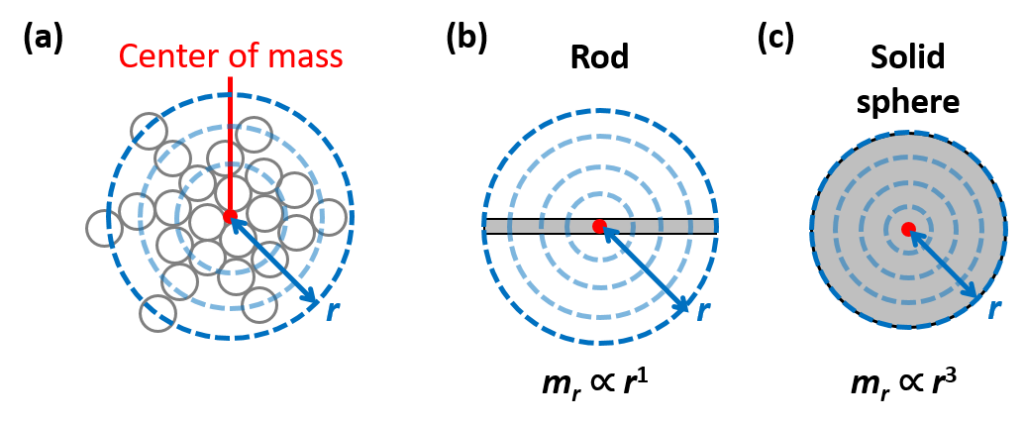
This approach is depicted for two limiting cases: a linear rod (Figure 3.5(b)), and a solid sphere (Figure 3.5(c)). From the diagram, it can be apparent that the mass enclosed within each radius [latex]{r}[/latex] is linearly related to [latex]{r}[/latex] for the rod; hence, [latex]{D}_{\text{f}}[/latex] is equal to 1. In contrast, [latex]{m}_{r}[/latex] is proportional to the volume enclosed by [latex]{r}[/latex] for the solid sphere, where the volume is fully occupied by the particle mass. The fractal dimension [latex]{D}_{\text{f}}[/latex] represents the exponent on [latex]{r}[/latex], as indicated in Equation 3.17.
| [latex]m\left( r \right)\propto\pi{{r}^{{{D}_{\text{f}}}}}[/latex] | Fractal dimension (3.17) |
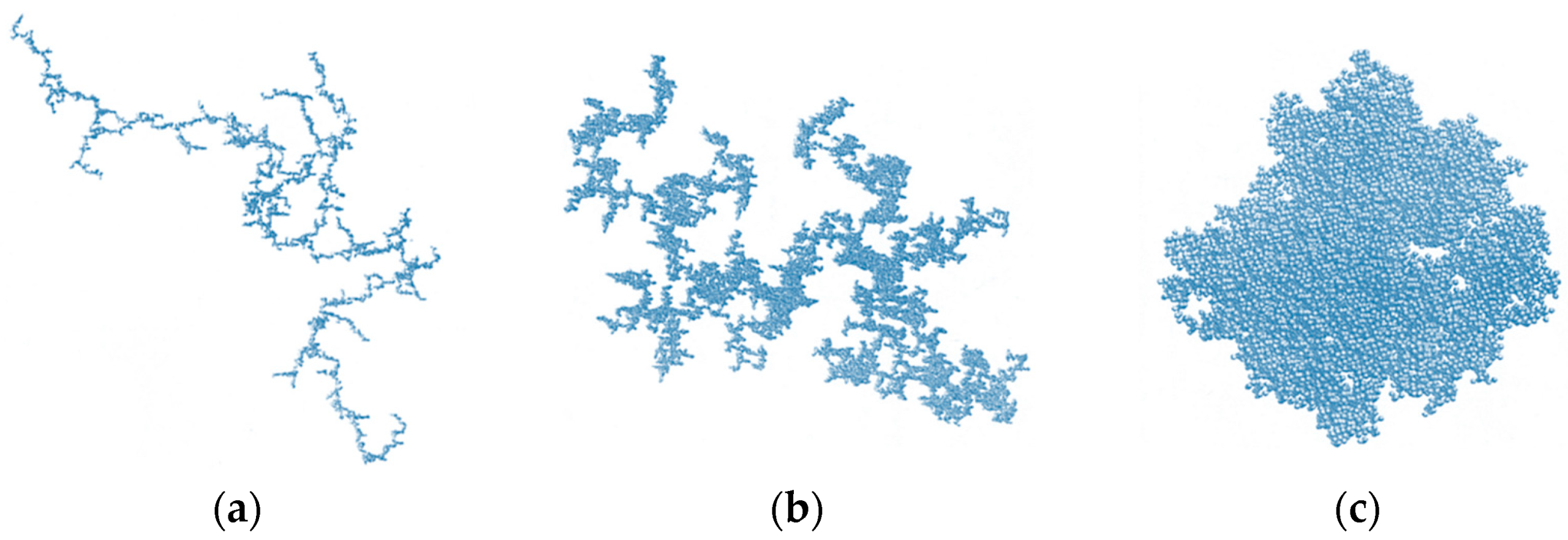
Figure 3.6 shows simulations of a suite of aggregate or agglomerate structures covering a range of fractal dimentions. It is apparent that [latex]{D}_{\text{f}}[/latex] is closer to 1 for loose structures (which are more rod-like), whereas [latex]{D}_{\text{f}}[/latex] is closer to 3 for dense structures (which are nearly solid spheres). Notably, the density of the agglomerate structure tends to depend on the attachment rate, as will be discussed in Chapter 7 on colloidal stability.
Interactive Question 3.2
The Certificate of Analysis for NIST Standard Reference Material® 1898 (Titanium Dioxide Nanomaterial) presents the following set of TEM and SEM images demonstrating three different levels of structure: individual crystallites with sizes < 50 nm (arrows on top image), fused particle structures with sizes ≈ 100 nm (middle images), and large clusters of particles with microscale sizes (bottom images) that can be fragmented into the smaller structures with energy input, e.g., sonication.
1. Drag and drop the terms “primary particle,” “agglomerate,” and “aggregate” to label the appropriate structure in the image.
The original version of this chapter contained H5P content. You may want to remove or replace this element.
2. Would you expect the fractal dimension for the structures in the bottom image to be closer to a value of 1 or 3?